activity_modeling_practice_nhanes – Introduction to Data Analytics and R Programming

Activity: EDA with health data from NHANES

Putting things together for exploratory data analysis.

This activity involves the NHANES package dataset which has 76 variables and 10000 observations, containing survey response data on health and nutrition.

NHANES survey data are collected by the US National Center for Health Statistics (NCHS) which has conducted a series of health and nutrition surveys since the early 1960’s. Since 1999, approximately 5,000 individuals of all ages are interviewed in their homes every year and complete the health examination component of the survey.

Part 1

Step 1

Tidyverse dplyr review

Write code to create a new data frame, nhanes, that contains data from NHANES for adults aged 26 to 64, inclusive, whose employment status, encoded in the variable Work, is known, i.e. is not NA. Age is encoded in the variable Age.

# Your code here

Step 2

Tidyverse dplyr review

The Work variable has only three values: NotWorking, Working, Looking. Write the code you would use to learn that those are the three values in the Work column.

# Your code here

Step 3

Tidyverse ggplot review

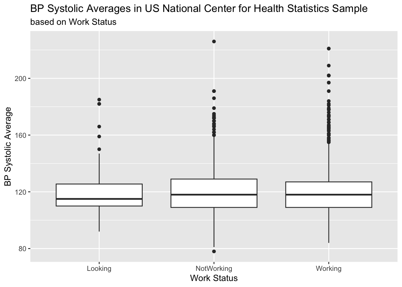
The variable BPSysAve gives the systolic blood pressure (the top number when blood pressure is measured). Write code that would generate the below visualization showing the relationship between systolic blood pressure and work status.

# Your code here

Step 4

Tidyverse dplyr Review

Continuing with the relationship between blood pressure and work status, describe the summary statistics you would need in order to describe the relationship shown in the above plot (e.g, what does the line in the box plot represent?). With code, compute those statistics.

# Your code here

Prepare for modeling

The variable SleepHrsNight indicates the number of hours people sleep per night. This is NA for some respondents. Below we run code that will overwrite nhanes with a new version that includes a new variable indicating whether a respondent gets a healthy amount of sleep, defined by the National Sleep Foundation as 7 to 9 hours per night for adults between the ages of 26 and 64. Here we don’t change the NA values.

nhanes <- nhanes %>% 
      mutate(sleep_health = case_when(     
                              SleepHrsNight <= 9 & SleepHrsNight >= 7 ~ "healthy", 
                              SleepHrsNight < 7 | SleepHrsNight > 9 ~ "unhealthy",
                              TRUE ~ as.character(SleepHrsNight))) #Since the new variable is character, we need to specify this when we reference the orignal numeric variable SleepHrsNight.

Using the updated data frame, we write code that will show the number and percentage of the respondents who fall into each sleeper group (the healthy and the unhealthy).

nhanes %>% 
  filter(!is.na(sleep_health)) %>% 
  count(sleep_health) %>% 
  mutate(percent=n/sum(n)*100)

Step 5

Tidyverse ggplot review

Using the most recent iteration of the nhanes data table, create scatterplots to compare the systolic blood pressure dependent variable with patient Age, DaysMentHlthBad, and BMI. As needed, use R to learn what each variable represents.

# Your code here

Step 6

Using the most recent iteration of your nhanes data table, write code to fit a regression model predicting systolic blood pressure from Age. In reality, many more variables are involved in predicting blood pressure, but we’ll keep it simple here.

# Your code here

Step 7

When I run my regression model, the output is

(Intercept) 101.3782

Age 0.4024

Write the corresponding equation and explain what this tells us about the relationship between systolic blood pressure and Age. Note that systolic blood pressure is measured in mm Hg (referring to millimeter of mercury, a unit of pressure).

Step 8

Now, let’s incorporate the newly created categorical variable indicating whether or not the individual gets a healthy amount of sleep. Add in the categorical variable as a predictor and run the linear model. Briefly summarize the result using complete sentences.

# Your code here

Step 9

What other categorical indicators might help explain blood pressure observations? Choose an additional categorical variable to include and run the model. Briefly summarize the result using complete sentences. Include a comment about how the model results change between models in Step 6, Step 8, and Step 9.

# Your code here

Part 2

Now it is your turn to conduct your own exploratory data analysis with NHANES data.

Step 10

Start by selecting a continuous dependent variable described in the NHANES R Documentation page. Select from the list: BMI or TotChol.

Create a histogram and box plot with that variable.

# Your code here

Step 11

Select and generate histograms for at least 2 possible numerical predictor variables that you think help explain your chosen dependent variable.

# Your code here

Step 12

Generate separate scatterplots describing your chosen dependent variable as a function of the explanatory variables you explored in the previous step. Create plots for at least 2 possible numerical predictor variables.

# Your code here

Step 13

Based on the plots you created above, is there one variable that seems to be most informative for predicting your dependent variable? Discuss your reasoning.

# Your code here

Step 14

Use the lm function to determine a linear model fit to predict your dependent variable based on one of your numerical explanatory variables you expect to have a strong association. Briefly describe the result. What can you say about the strength of the linear relationship between the x and y variable?

# Your code here

Step 15

Given the results of the previous step, write out the equation that represents the model for predicting your dependent variable from one of your explanatory variables. Store the result in an object estimate.

# Your code here

Step 16

Calculate the required variables and make a scatter plot which shows the residuals \(e_i = y_i - \widehat{y_i}\) on the y-axis and the predicted values \(\widehat{y_i}\) on the x-axis.

What aspects of the residual plot show that the linear model is appropriate or not? Are there any aspects of the residual plot that cause you to be concerned about the fitting of the linear model? Add your response in your Quarto.

# Your code here