What is a Model?

Intro to Data Analytics

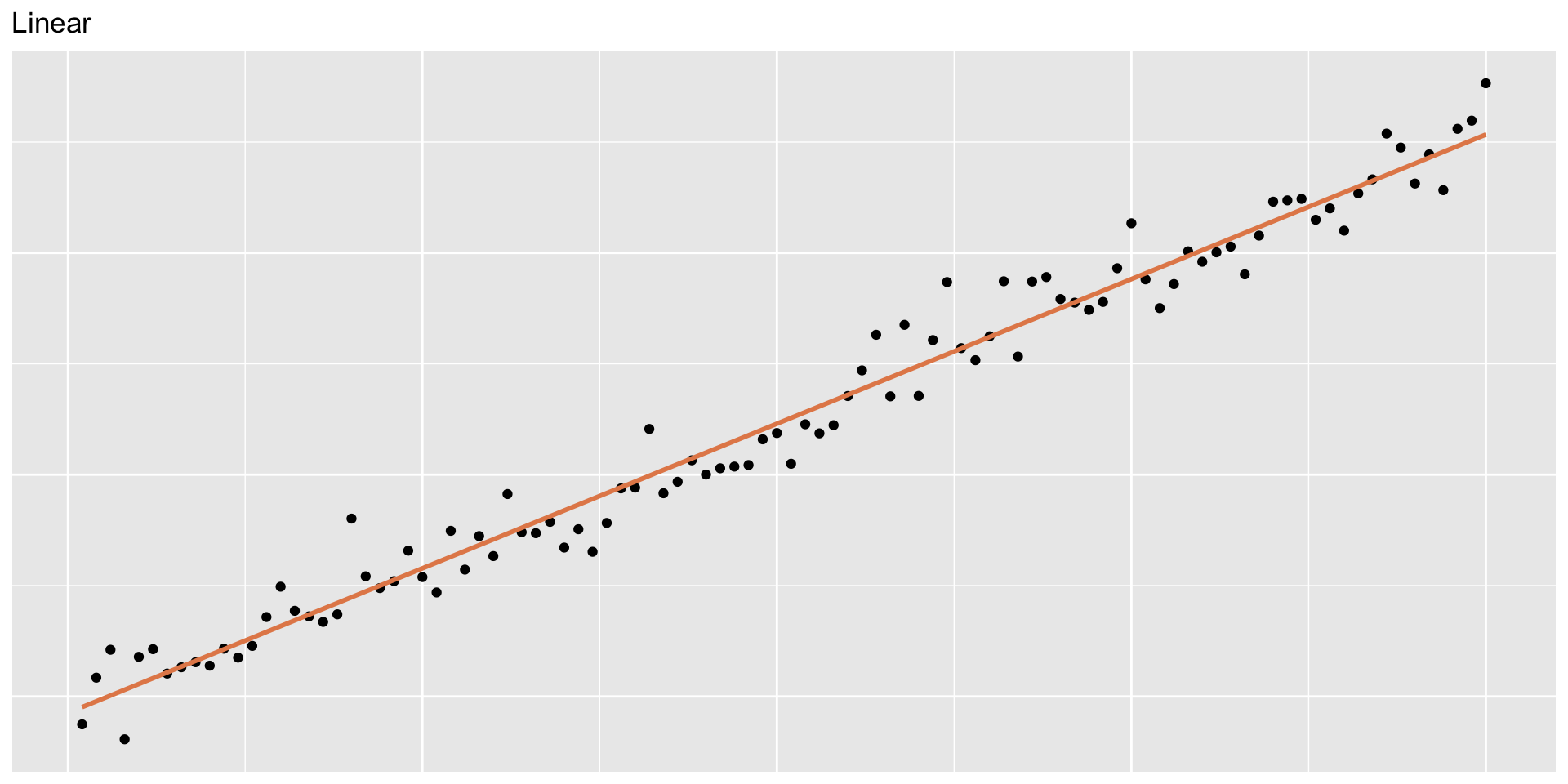
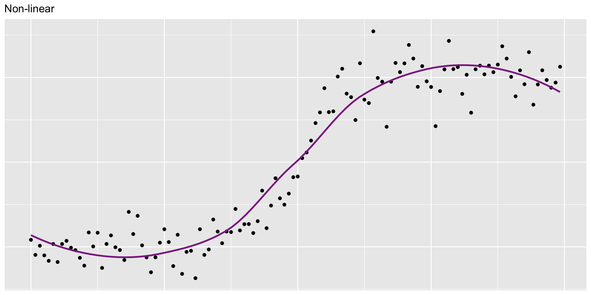
Models

• Use models to explain relationships (between variables)
  • Linear vs. nonlinear

How do we use models?

• Explanation – Characterize relationship between y and x by using
  • slope for numerical explanatory variables
  • differences for categorical explanatory variables
• Prediction – plug in x, get predicted y

Models

• Simple terms:
  • Width vs. height (of paintings, furniture, etc.)

Note

Download the data used in these slides.

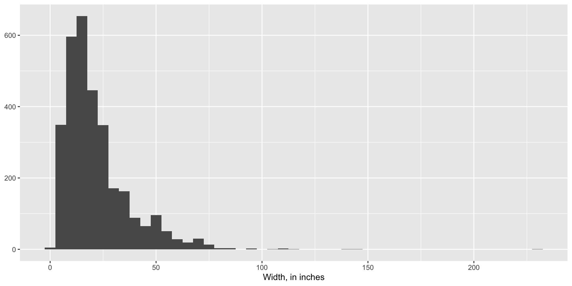
Continuous Data Distribution

Width

ggplot(data = paintings, aes(x = Width_in)) +
  geom_histogram(binwidth = 5) +
  labs(x = "Width, in inches", y = NULL)

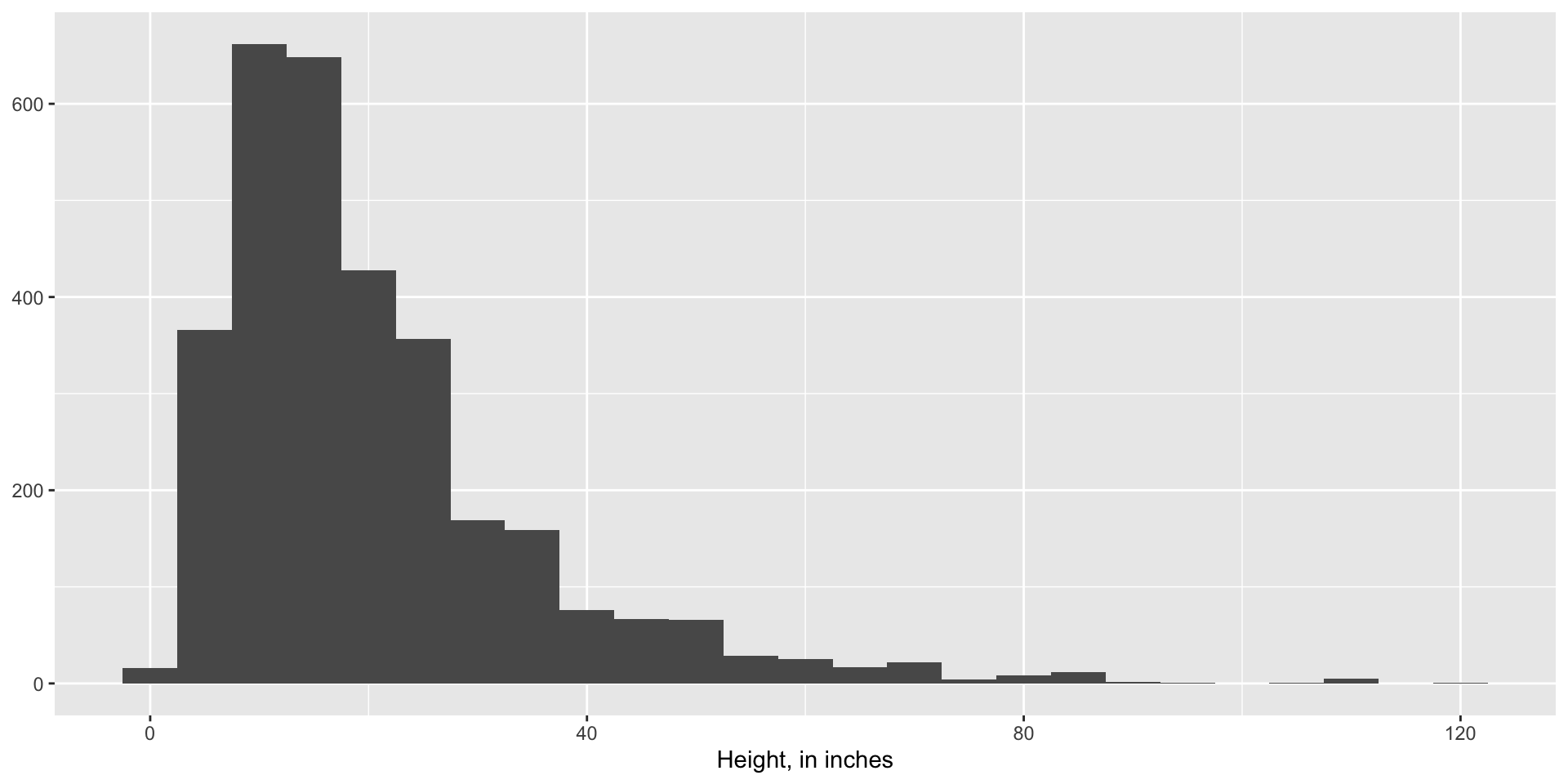
Continuous Data Distribution

Height

ggplot(data = paintings, aes(x = Height_in)) +
  geom_histogram(binwidth = 5) +
  labs(x = "Height, in inches", y = NULL)

Reminder

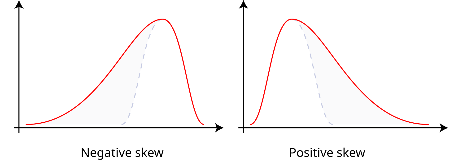
• Positive skew: The right tail is longer; the mass of the distribution is concentrated on the left of the figure. The distribution is said to be right-skewed, right-tailed, or skewed to the right, despite the fact that the curve itself apaintingsears to be skewed or leaning to the left; right instead refers to the right tail being drawn out and, often, the mean being skewed to the right of a typical center of the data.
• Negative skew: The left tail is longer; the mass of the distribution is concentrated on the right of the figure. The distribution is said to be left-skewed, left-tailed, or skewed to the left

Models

• Can think about this as a relationship between width and height as a function
• Function might look like this
  • y = 4x + 8
• Or like this
  • height = b * width + e
  • b is the slope –> what we care about

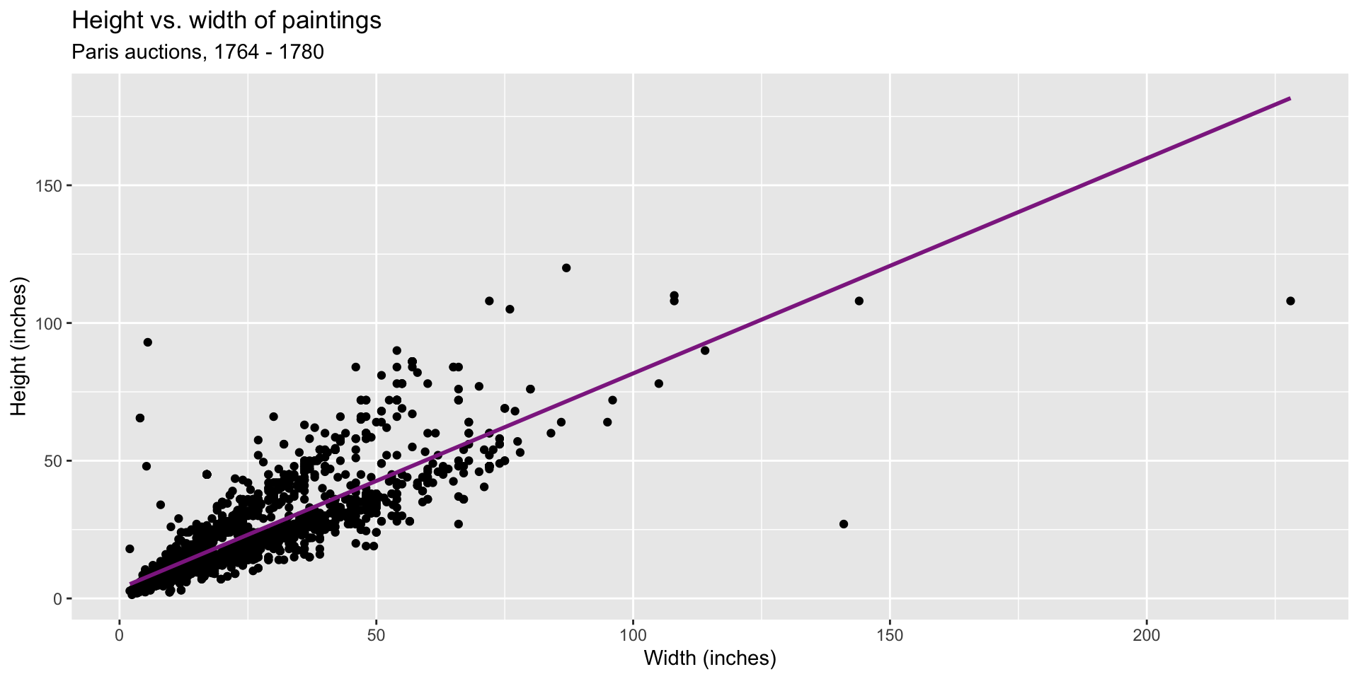
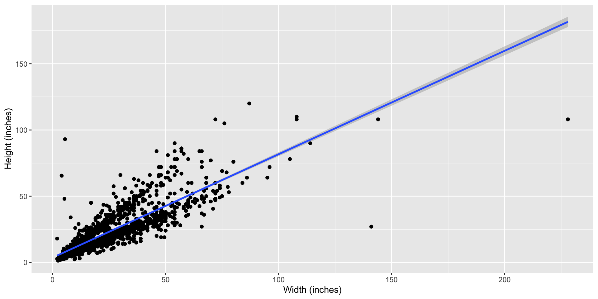
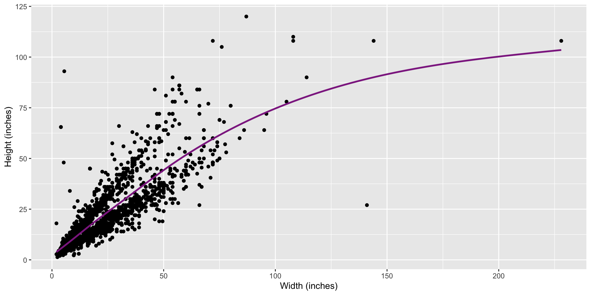
Height as a function of width

Height as a function of width

ggplot(data = paintings, aes(x = Width_in, y = Height_in)) +
  geom_point() +
  geom_smooth(method = "lm") +
  labs(
    x = "Width (inches)",
    y = "Height (inches)"
  )

Models other functions

Models other functions

ggplot(data = paintings, aes(x = Width_in, y = Height_in)) +
  geom_point() +
  geom_smooth(method = "gam", #<<
              se = FALSE, color = "#8E2C90") + 
  labs(
    x = "Width (inches)",
    y = "Height (inches)"
  )

• gam stands for generalized additive model. A statistical model that explains a response (dependent variable, y) by adding up smooth, non-linear functions of the predictor variables (x).

Model Terminology

• Response variable (target/dependent variable)

• Predictor variable (independent/explanatory variable)

• Predicted value (typical or expected value of response variable)

• Residuals (distance between predicted value and observed)

Model Terminology

• Response variable (target/dependent variable)
  • y-axis – variable whose behavior you are trying to understand

• Predictor variable (independent/explanatory variable)
  • x-axis – variables you want to use to explain variation in response

• Predicted value – output of the model function
  • function gives typical (expected) value of response variable conditioning on explanatory variable

• Residuals - measure of how far each case is from predicted value
  • Residual = Observed value - Predicted value
  • how far above/below expected value each case is

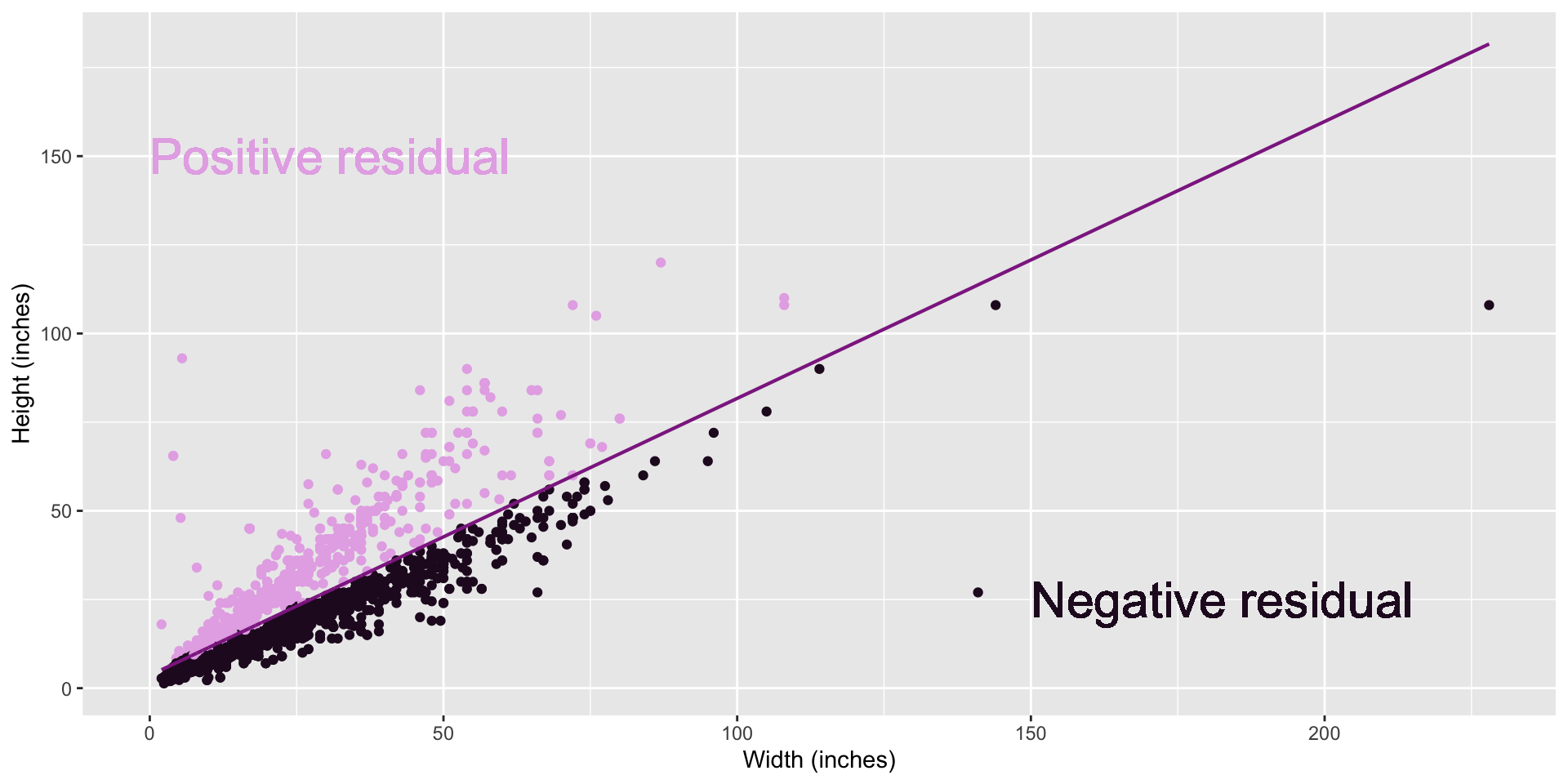
Residuals

Predictors

Model pros/cons

• Pros: good at describing global relationships, big picture
  • might reveal patterns we don’t see in visual inspection of data
• Cons: might impose a structure that’s not really there in the data

How do we use models?

• Explanation – Characterize relationship between y and x by using
  • slope for numerical explanatory variables
  • differences for categorical explanatory variables
• Prediction – plug in x, get predicted y

Models with numerical explanatory variables

Data: Paris Paintings

• Number of observations: 3393
• Number of variables: 61

Goal: Predict height from width

\[\widehat{height}_{i} = \beta_0 + \beta_1 \times width_{i}\]

Troubleshooting: Installing tidymodels

What to do if you face an error when installing and loading the tidymodels package.

• The newest version of tidymodels might require you to update the rlang package. Use install.packages("rlang") to update.
• A small chance, but it is also possible that you will need to update your version of RStudio (see the Getting Started resources from the beginning of the semester)