Join exercises with baby names and books

Create a new Quarto titled “join_review_yourname.qmd” to record your work on the activity. You do not need to submit this on Brightspace, but you are welcome to share your Quarto with me over email for feedback.

Load the required packages: tidyverse and babynames

How to use this page:

In Part 1 and Part 2, the solution code is not automatically displayed, but you can see it by clicking the Code buttons. This gives you the opportunity to think first about how something should be done and then check to see what code was actually used. I strongly recommend you take the time to attempt an answer the question before revealing the solution.
Part 3 gives you a chance to apply what you’ve learned about joins in exercises without example solutions.

Part 1: dplyr review

Baby Names

The babynames data frame contains full baby name information provided by the U.S. Social Security Administration. The data frame has 5 variables:

Code

names(babynames)

[1] "year" "sex"  "name" "n"    "prop"

where n is the number of occurrences of that name for that sex in that year, and prop is n divided by the total number of applicants in that year – so it is the proportion of people born in that year with that sex and name. In other words, consider the first row of the data frame:

Code

babynames %>% head(1)

# A tibble: 1 × 5
   year sex   name      n   prop
  <dbl> <chr> <chr> <int>  <dbl>
1  1880 F     Mary   7065 0.0724

which tells us that in 1880 there were 7065 girl babies named Mary and that was 7.24% of babies born that year!

Step 1

Update the babynames data frame by adding a new variable called popular that will be TRUE if the name was assigned to more than 1% of all babies in that year.

Code

babynames <- babynames %>% mutate(popular = (prop > .01))

# OR 
babynames <- babynames %>% mutate(popular = if_else(prop>.01, TRUE, FALSE))

Step 2

Write code that will show the 10 baby names that were the most popular in any single year (we’re not trying to aggregate across years). Note: the same name may appear multiple times in this output.

Code

babynames %>% 
  arrange(desc(prop)) %>% 
  head(10)

Step 3

We are interested in knowing which year had the greatest number of births. Write code that will show the data in descending order by number of births in each year.

Code

babynames %>% 
  group_by(year) %>%
  summarize(n = sum(n)) %>%
  arrange(desc(n))

Part 2: Joins

For Part 2, try the code in your Quarto while you work through the examples.

Preparing for joins

In the babynames package there is a table called births. It has just two columns:

Code

head(births)

# A tibble: 6 × 2
   year  births
  <int>   <int>
1  1909 2718000
2  1910 2777000
3  1911 2809000
4  1912 2840000
5  1913 2869000
6  1914 2966000

These data come from the U.S. Census Bureau (see help(births) for more information). For clarity, let’s put this table into a new object with a better name.

Code

census_births <- births

The information about individual names is stored in the babynames table. These data come from the Social Security Administration (see help(babynames) for more details). We expect that the total number of births recorded by the Census Bureau should match the total number of births as recorded by the Social Security Administration, but let’s investigate this.

First we should condense the SSA data into the same yearly form as the Census Bureau data. We can do this with group_by and summarize. Think about how to do this, and try it out in your Quarto, before you look at the code.

Reminder: the n() function counts the number of observations in a group. It can only be used in the summarize, mutate, and filter functions.

Code

ssa_births <- babynames %>%
  group_by(year) %>%
  summarize(N = n(), births = sum(n))

Actually, I’m going to make one small change. In order to make the subsequent exercises more interesting, I’m going to repeat the above but filter to exclude data from 2012 on so that the tables don’t end in the same year.

Code

ssa_births <- babynames %>%
  filter(year < 2012) %>%
  group_by(year) %>%
  summarize(N = n(), births = sum(n))

Now I have two separate tables with what should be the same information: census_births and ssa_births, but they don’t cover the same set of years. We can see this by doing some summarizing of both tables.

Code

census_births %>%
  summarize(
    N = n(),
    earliest = min(year),
    latest = max(year)
  )

# A tibble: 1 × 3
      N earliest latest
  <int>    <int>  <int>
1   109     1909   2017

Code

ssa_births %>%
  summarize(
    N = n(),
    earliest = min(year),
    latest = max(year)
  )

# A tibble: 1 × 3
      N earliest latest
  <int>    <dbl>  <dbl>
1   132     1880   2011

Joins

As you know, we can combine two data frames with a join operation. Generally we want to in some way match rows in one data frame rows that correspond in a different data frame.

If we use an inner_join the result will have only rows that have a corresponding match in both of the data frames.

Code

census_births %>%
  inner_join(ssa_births, by = "year") %>%
  summarize(
    N = n(),
    earliest = min(year),
    latest = max(year)
  )

# A tibble: 1 × 3
      N earliest latest
  <int>    <dbl>  <dbl>
1   103     1909   2011

You can see that the set of years that results is the intersection of the two sets of years in the original data frames.

If we use a left_join then we will get all the rows from census_births, even if there is no corresponding entry in the ssa_births table. This means that rows that have no corresponding entry will get NAs in place of the missing data.

Code

total_births <- census_births %>%
  left_join(ssa_births, by = "year")

total_births %>%
  filter(is.na(births.y))

# A tibble: 6 × 4
   year births.x     N births.y
  <dbl>    <int> <int>    <int>
1  2012  3952841    NA       NA
2  2013  3932181    NA       NA
3  2014  3988076    NA       NA
4  2015  3978497    NA       NA
5  2016  3945875    NA       NA
6  2017  3855500    NA       NA

By using a filter for the NA data, I can see that the data from 2012 onward exists in the census_births data frame, but not in the ssa_births data frame. Obviously, this is no longer the intersection of the two data frames.

Code

total_births %>%
  summarize(
    N = n(),
    earliest = min(year),
    latest = max(year)
  )

# A tibble: 1 × 3
      N earliest latest
  <int>    <dbl>  <dbl>
1   109     1909   2017

We can easily see that a right_join will have the opposite effect. There are many years of SSA data that have no match in the Census data and we can see that by looking for the data that has NAs.

Code

total_births <- census_births %>%
  right_join(ssa_births, by = "year")

total_births %>%
  filter(is.na(births.x))

# A tibble: 29 × 4
    year births.x     N births.y
   <dbl>    <int> <int>    <int>
 1  1880       NA  2000   201484
 2  1881       NA  1935   192696
 3  1882       NA  2127   221533
 4  1883       NA  2084   216946
 5  1884       NA  2297   243462
 6  1885       NA  2294   240854
 7  1886       NA  2392   255317
 8  1887       NA  2373   247394
 9  1888       NA  2651   299473
10  1889       NA  2590   288946
# ℹ 19 more rows

The number of years represented is neither the intersection, nor the union of the original data frames.

Code

total_births %>%
  summarize(
    N = n(),
    earliest = min(year),
    latest = max(year)
  )

# A tibble: 1 × 3
      N earliest latest
  <int>    <dbl>  <dbl>
1   132     1880   2011

Keep in mind that if you switch the order of the data frames and switch back to left_join you get exactly the same results. In other words, left_join(a, b) is the same as right_join(b, a).

Code

ssa_births %>%
  left_join(census_births, by = "year") %>%
  summarize(
    N = n(),
    earliest = min(year),
    latest = max(year)
  )

# A tibble: 1 × 3
      N earliest latest
  <int>    <dbl>  <dbl>
1   132     1880   2011

This brings us to full_join which results in all rows, regardless of whether or not thaty are matched.

Code

total_births <- census_births %>%
  full_join(ssa_births, by = "year")

total_births %>%
  filter(is.na(births.x) | is.na(births.y))

# A tibble: 35 × 4
    year births.x     N births.y
   <dbl>    <int> <int>    <int>
 1  2012  3952841    NA       NA
 2  2013  3932181    NA       NA
 3  2014  3988076    NA       NA
 4  2015  3978497    NA       NA
 5  2016  3945875    NA       NA
 6  2017  3855500    NA       NA
 7  1880       NA  2000   201484
 8  1881       NA  1935   192696
 9  1882       NA  2127   221533
10  1883       NA  2084   216946
# ℹ 25 more rows

Now the set of years that results really is the union of the years in the two data frames.

Code

total_births %>%
  summarize(
    N = n(),
    earliest = min(year),
    latest = max(year)
  )

# A tibble: 1 × 3
      N earliest latest
  <int>    <dbl>  <dbl>
1   138     1880   2017

Data Reconciliation

Let’s take a look ahead at the stats package to help us understand the relationship between these two datasets.

Once we have the data frames joined, we can compare the birth numbers directly. I’ll use the cor function which calculates the correlation between two vectors (it’s in the stats package). While the birth numbers are strongly correlated…

Code

total_births %>%
  summarize(
    N = n(),
    correlation = cor(births.x, births.y,
      use = "complete.obs"
    )
  )

# A tibble: 1 × 2
      N correlation
  <int>       <dbl>
1   138       0.892

the numbers are not the same.

Code

library(ggplot2)
ggplot(data = total_births, aes(x = year, y = births.x)) +
  geom_line() +
  geom_line(aes(y = births.y))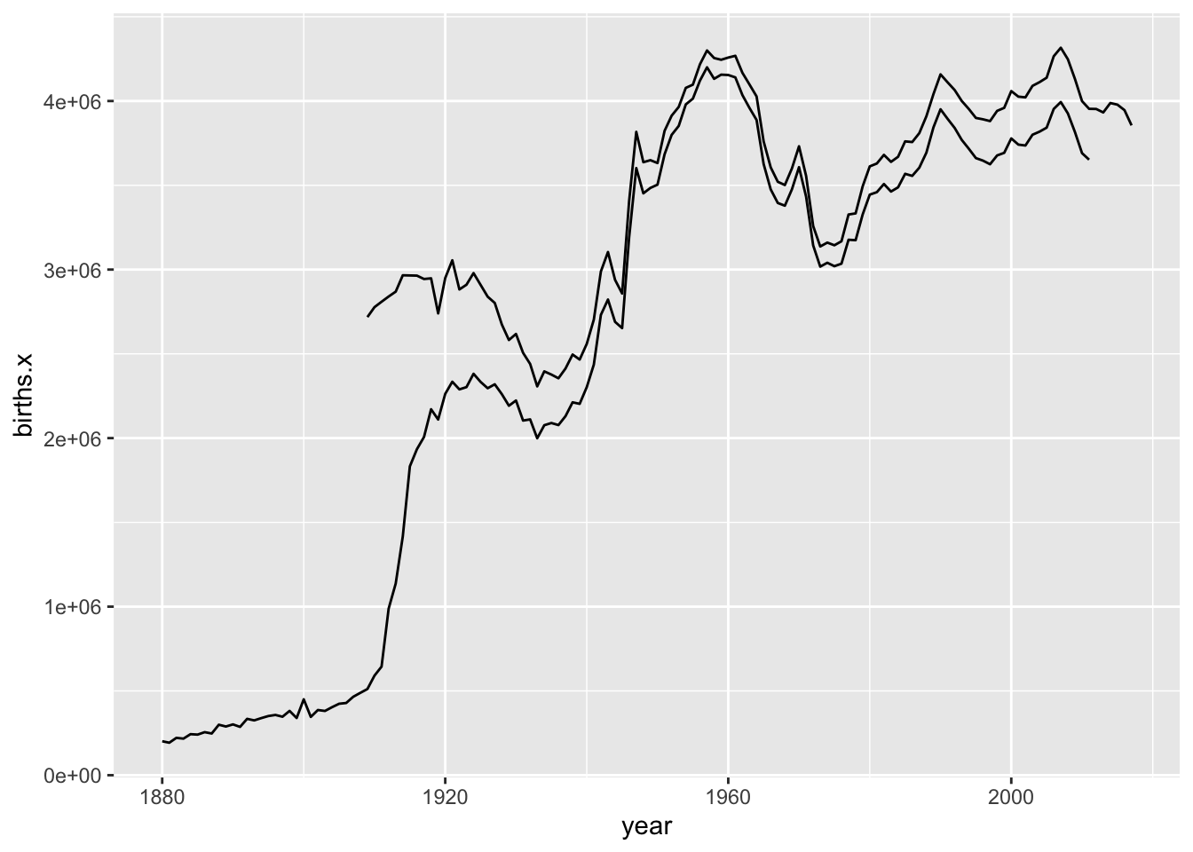

A deeper dive into the documentation for babynames might help you figure out why.

Part 3: Joins with Books and authors data tables

Now it’s your turn to practice joins without the Code example solutions. You will load the required data tables from a GitHub repository storing the .csv files (see below for directions).

The files books.csv, authors.csv, and book-authors.csv give details about the planned summer reading of a statistics student. books.csv provides details for each book (isbn, title, year, and genre), authors.csv provides details about each author (authorid, first name, last name, and nationality), and book-authors.csv provides the author identification (authorid) for each isbn (books with multiple authors will have multiple rows).

For Part 3, run the following code to prevent the use of scientific notation:

Code

options(scipen=999)

Step 1

Read the three files into R, naming them books, authors, and book_authors. To read in the datasets below from GitHub, place the entire url inside of the read_csv() function.

Code

# Your code here

Step 2

Use the appropriate *_join statement to add the ISBNs to the authors data table. Create a new object with the result, use a descriptive name like authors_isbn. Make a note of why you chose this particular join function in the code chunk.

Remember that join keys need either need to have precisely the same name, or you need to add an argument to tell R which variables hold the join key.

Why does the resulting data frame have 31 rows instead of 11? Take a look at the tables to determine what happened. Include your response to the question in a comment inside your code chunk.

Code

# Your code here

Step 3

To eliminate the duplicate rows of your data frame from Step 2, which we’ll assume you named authors_isbn, run the following code. Remember to change the object names to align with your code as necessary.

authors_isbn <- unique(authors_isbn)

Code

# Your code here

Step 4

Use the appropriate *_join statement to add the author information table from Step 3 to the books data table. Create a new object with the result. Make a note of why you chose this particular join function in the code chunk.

Code

# Your code here

Step 5

Are there any authors in the authors data table that do not correspond to the books that are included in the books data table? Use an appropriate filtering join statement to do this. Make a note of why you chose this particular join function in the code chunk.

Code

# Your code here

Step 6

After reading A Game of Thrones the student decides to read the rest of the series over the summer. books2.csv contains the updated books on the student’s reading list. Read this file into R, naming it books2.

books.csv is available at: https://raw.githubusercontent.com/ds4stats/r-tutorials/master/merging/data/books2.csv

Code

# Your code here

Step 7

Use the same join statement that you used in Step 4, but using books2 rather than books. Make a note of why you chose this particular join function in the code chunk.

Code

# Your code here