Install R and R Studio for Windows

Lab instructions for Windows computers

These instructions apply to Windows computers only. If you are not using a Windows computer, please return to the previous page and choose the correct computing device from the list.

Installing new software

You are about to install two separate programs: R, the programming language that does the computing, and RStudio, the IDE you drive it from. Getting Started explains why you need both, review that page first if you have not yet done so.

The short version: R is the engine, RStudio is the dashboard. Install R first, RStudio second, and from then on you will only ever open RStudio.

Follow the instructions below to install both, and then verify your installation is set up correctly.

At the end of this activity, you will submit an .html file for completion credit. You can make multiple submissions, as needed.

Step 1: Install R

R is a programming language and computing environment specialized for statistical analysis and data manipulation. It’s commonly used for performing statistical tests, creating data visualizations, and writing data analysis reports. Despite focusing on statistics, it’s a full-fledged programming language, and relatively easy to learn.

Go to https://cloud.r-project.org/bin/windows/base/, and click the link titled Download R-4.6.1 for Windows.

This will download the R installer to your computer’s download folder. Go to your download folder, and double-click on the R-4.6.1 installer you just downloaded. Follow the prompts on the screen to finish installing R. You can safely accept all the default settings without changing anything.

If you want to see more visually detailed instructions for how to install R, you can watch this video tutorial.

Note that some of the software versions number might change (for example, a later release such as R 4.7 instead of R 4.6.1), but the steps you should follow will be exactly the same.

Step 2: Install RStudio

RStudio is an integrated development environment for reproducible scientific computing that supports the R programming language.

Instructions

Download the latest, free version of RStudio Desktop. Be sure to get the version that is appropriate for your operating system.
Install RStudio Desktop by launching the installer after it downloads. You can accept all the defaults during installation.

If you want to see more visually detailed instructions for how to install RStudio, you can watch this video tutorial

Note that some of the software versions number might change, the steps you should follow will be exactly the same.

Verification

Next, let’s open RStudio, to verify that R and RStudio have been installed correctly. Here is what you should do to open RStudio:

Click the Windows Start button in the taskbar
Scroll through the alphabetical list of installed programs until you find RStudio
Click on RStudio to open it. Be sure to click the icon for RStudio, not the icon for R.

If you can’t locate it this way, type RStudio into the search box next to the Start button.

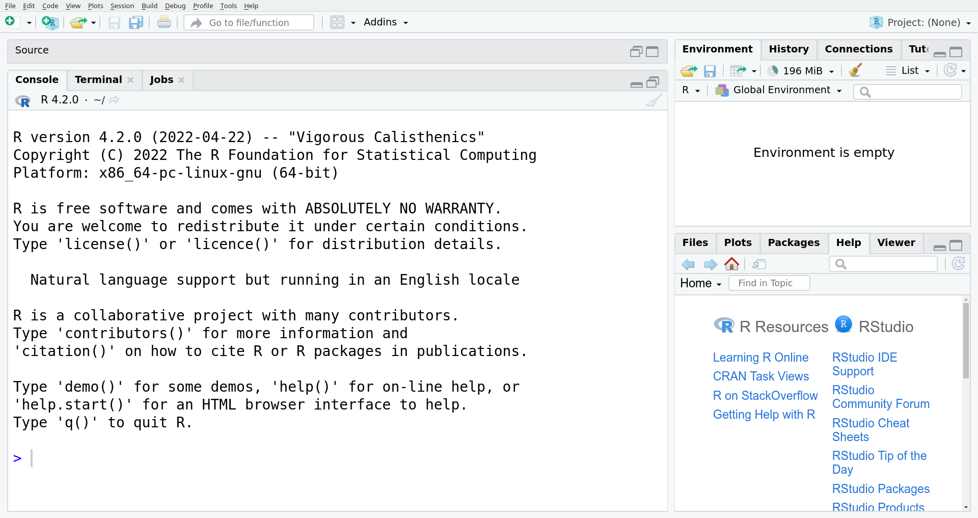
When RStudio opens, you should see a window that looks something like this:

Sometimes, RStudio cannot be installed. For example, if the operating system is out of date, or you do not have enough space on the computer’s hard drive to fit the program. If RStudio cannot be installed on your computer, please notify me.

A tour of the RStudio interface

Now that RStudio is open in front of you, here is what you are looking at. The window is divided into panes:

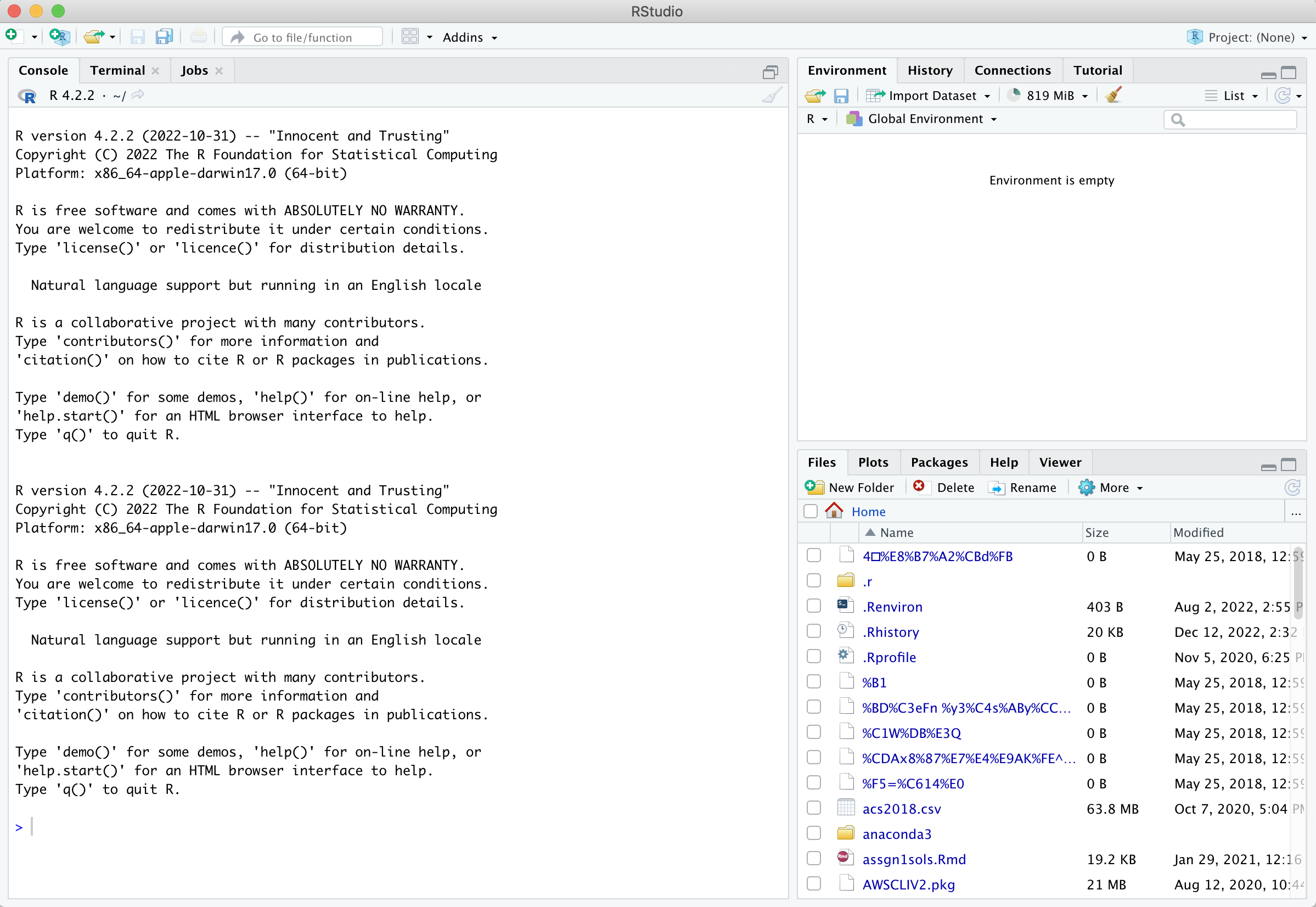
Console (left) - The way R works is you write a line of code to execute some kind of task on a data object. The R Console allows you to run code interactively. The screen prompt > is an invitation from R to enter its world. This is where you type code in, press enter to execute the code, and see the results.
Environments: Environment, History, and Connections tabs (upper-right)
- Environment - shows all the R objects that are currently open in your workspace. This is the place, for example, where you will see any data you’ve loaded into R. When you exit RStudio, R will clear all objects in this window. You can also click on to clear out all the objects loaded and created in your current session.
- History - shows a list of executed commands in the current session.
- Connections - you can connect to a variety of data sources, and explore the objects and data inside the connection. I typically don’t use this window, but you can.
Output: Files, Plots, Packages, Help and Viewer tabs (lower-right)
- Files - shows all the files and folders in your current working directory (more on what this means later).
- Plots - shows any charts, graphs, maps and plots you’ve successfully executed.
- Packages - tells you all the R packages that you have access to (more on this later).
- Help - shows help documentation for R commands that you’ve called up.
- Viewer - allows you to view local web content (won’t be using this much).
Source
- The source pane allows users to view and edit various code-related files, such as .R, .rmd, .qmd, .py, .css, or general text files such as .txt or .md. By default it is the top-left panel and can be launched by opening any editable file in RStudio. Each additional file that is opened will be added as a new tab within the Source pane.

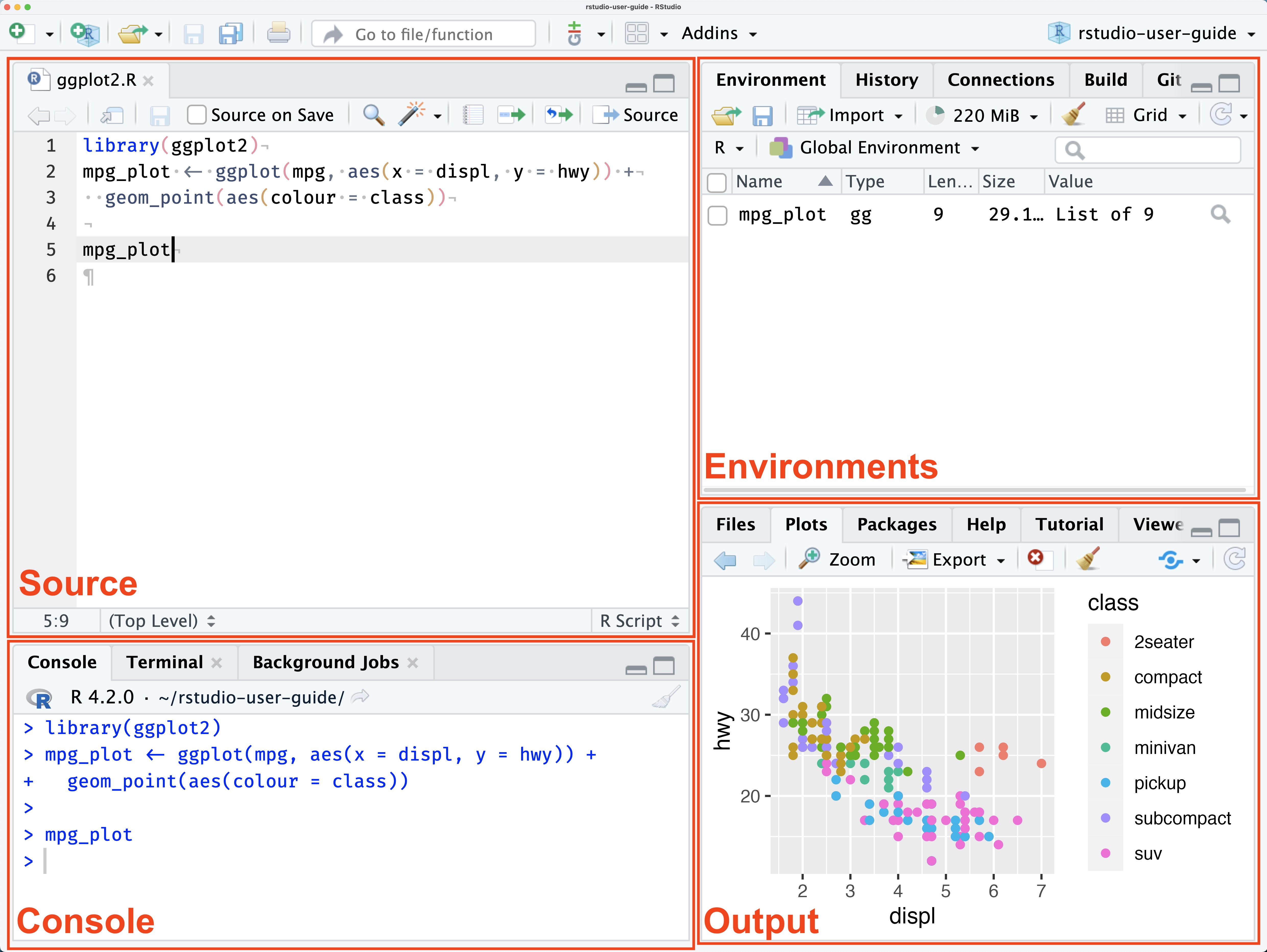
Running R code using the console (bottom left in figure below) is a great place to start, but has its limitations. Each time you want to execute a set of commands, you have to re-enter them at the command line. Complex commands are potentially subject to typographical errors, necessitating that they be re-entered correctly. Repeating a set of operations requires re-entering the code stream. To give yourself more room to work, it’s a great idea to use the R script editor in the Source pane.

A script is simply a text file containing a set of commands and comments. The script can be saved and used later to re-execute the saved commands. The script can also be edited so you can execute a modified version of the commands.

You can open a new empty script by clicking the New File icon in the upper left of the main RStudio toolbar. This icon looks like a white square with a white plus sign in a green circle. Clicking the icon opens the New File Menu. Click the “R Script” option and the script editor will open with an empty script in the Source pane. Your R Studio should look similar to below (image source: R for Data Science)

R Markdown documents take script files to a new level by allowing you to mix R commands with explanatory text. Think of an R Markdown document as an R script on steroids. Your R Markdown source document is compiled into an output report evaluating the R commands in the source document to produce easily reproducible results in an aesthetically pleasing form. It combines code, results from the code, and narrative text explaining the results to produce beautiful documents and academic reports.

Installing R packages

Like many modern programming languages, R is modular, meaning that it relies on packages to provide additional functionality. There are thousands of R packages hosted on CRAN, and many more hosted on GitHub. In this course, we will focus on a handful of popular, well-crafted, useful packages.

In RStudio, the Packages tab displays a searchable list of packages that are installed on your computer.

You should get comfortable checking which packages you have installed, and installing new packages. You only have to install a package once on your computer.

Install `rstudio.prefs` and customize your RStudio

RStudio has hundreds of options that can be configured so that each user can customize its behavior to their preferences. Unfortunately, several of its configuration options have default settings that make it more difficult to conduct reproducible data analyses. These settings can be changed using the Global Options graphical user interface (GUI), but hunting down each setting and changing them one at a time is slow and tedious.

Instead, we’ll use the rstudio.prefs package, which will allow use to change all the settings at once by executing a few R commands in the console. But first, we need to install the rstudio.prefs package.

Instructions

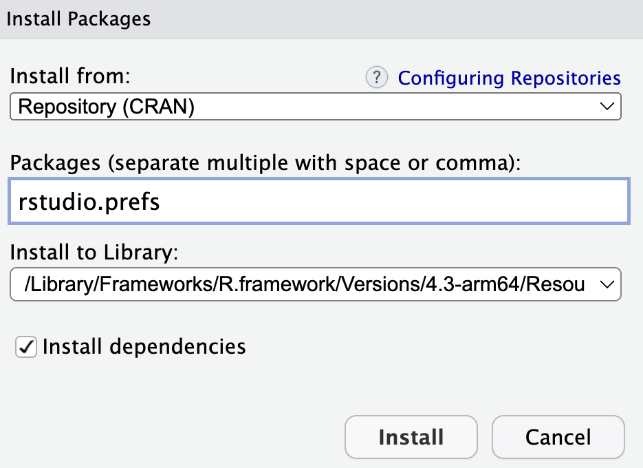
To install the rstudio.prefs package:

Open the “Packages” tab in the bottom-right pane of RStudio, and click the “Install” button along the top menu bar.

Make sure the “Install from:” drop down is set to Repository (CRAN)

In the pop-up window, type rstudio.prefs into the text box, and press the Install button to start the package installation. It should look something like this:

Configure RStudio
- Note: these steps are covered using a manual point-and-click process here.

Copy and paste the code below into the console (the “Console” is a tab in the window on the bottom left of the RStudio interface), and press the Enter key to run the code. This code will change several of RStudio’s default configuration options to make the program more user-friendly.

Before changing your settings, R will print out your pending changes, and ask if you want to continue. You can indicate “Yes” by typing a y into the console, and pressing the Enter key.

library(rstudio.prefs)

use_rstudio_prefs(
  save_workspace = "never",
  load_workspace = FALSE,
  restore_last_project = FALSE,
  restore_source_documents = FALSE,
  check_for_updates = FALSE,
  color_preview = FALSE,
  rmd_viewer_type = "pane",
  rmd_chunk_output_inline   = FALSE
)

If you get an error message in your console saying Error in library(rstudio.prefs) : there is no package called ‘rstudio.prefs’, return to Step 1 in this list and make sure you have finished installing the rstudio.prefs package.

Verification

Copy and paste the R code below into the console and press the Enter key to run the code. If you have configured RStudio correctly by following the instructions above, you should see a message that says “✔ RStudio is correctly configured!”.

rstudio_config <- jsonlite::fromJSON(paste0(rstudio.prefs::rstudio_config_path(),
                                            "/rstudio-prefs.json")
                                     )
options_set <- c(
  rstudio_config$save_workspace == "never",
  rstudio_config$load_workspace == FALSE,
  rstudio_config$restore_last_project == FALSE,
  rstudio_config$restore_source_documents == FALSE,
  rstudio_config$check_for_updates == FALSE,
  rstudio_config$color_preview == FALSE,
  rstudio_config$rmd_viewer_type == "pane",
  rstudio_config$rmd_chunk_output_inline == FALSE
  )

if (all(options_set)) {
  cli::cli_alert_success("RStudio is correctly configured!")
} else {
  cli::cli_alert_danger("RStudio settings have not been correctly configured.")
}

Install the course packages

The tidyverse is a meta-package that installs eight other commonly-used R packages. It is a popular way to use R (Wickham et al. 2019), and we will use it extensively. The rest of the list below holds packages we need later in the semester, or datasets our textbooks use:

Package	What it is for
`tidyverse`	the core toolkit for the whole course
`usethis`	project setup; we use it in this lab to check yours
`rmarkdown`	lets Quarto run the R code in your documents
`nycflights13`	flight data used throughout R4DS Chs. 3, 19 and 25
`palmerpenguins`, `ggthemes`	used in R4DS Ch. 1
`dslabs`	datasets from IDS, our main textbook
`openintro`	datasets from IMS

Instructions

Copy the code below, paste it into the console, and press the Enter key. This installs all of them at once. It will print a lot of output and may take a few minutes — that is normal.

install.packages(c("tidyverse", "usethis", "rmarkdown",
                   "nycflights13", "palmerpenguins", "ggthemes",
                   "dslabs", "openintro"))

This is the same install.packages() command you will see at the top of most R4DS chapters, so it is worth getting used to. You can also install packages by clicking through the Packages pane, the way you just did for rstudio.prefs — the two do exactly the same thing.

Verification

Copy and paste the R code below into the console and press the Enter key to run the code. If an appropriate version of the tidyverse package is properly installed, you should see two messages: “✔ tidyverse is installed and relatively up-to-date” and “✔ usethis is installed.”

has_tidyverse <- suppressPackageStartupMessages(require(tidyverse))
has_usethis <- suppressPackageStartupMessages(require(usethis))

if (has_tidyverse) {
  tidyverse_version <- packageVersion("tidyverse")

  if (tidyverse_version >= "2.0.0") {
    cli::cli_alert_success("tidyverse is installed and relatively up-to-date.")
  } else {
    cli::cli_alert_danger("tidyverse is installed but it is not up-to-date. Please update your packages.")
  }
} else {
  cli::cli_alert_danger("tidyverse could not be loaded.")
}
if (has_usethis) {
  cli::cli_alert_success("usethis is installed")
} else {
  cli::cli_alert_danger("usethis could not be loaded.")
}

Check that `rmarkdown` is ready

Quarto uses the rmarkdown package (and knitr, which installs alongside it) to run the R code inside your Quarto documents. Without it, the Render button will fail. It came in with the command above; this confirms it.

Verification

Copy and paste the R code below into the console and press the Enter key to run the code. You should see “✔ rmarkdown is installed — you can render Quarto documents.”

has_rmarkdown <- requireNamespace("rmarkdown", quietly = TRUE)

if (has_rmarkdown) {
  cli::cli_alert_success("rmarkdown is installed — you can render Quarto documents.")
} else {
  cli::cli_alert_danger('rmarkdown is not installed. Run install.packages("rmarkdown") in the console.')
}

Install `dsbox`

dsbox holds several datasets we will use later in the semester, including the Berkeley admissions data, the General Social Survey extract, and the DC bikeshare data.

This one is not installed the usual way

dsbox is not on CRAN, so install.packages("dsbox") will fail with a message saying the package “is not available for this version of R”. That message does not mean anything is wrong with your R installation. This package is distributed from GitHub instead, which takes one extra step.

Instructions

Paste both lines below into the console, one at a time. The first installs a small helper package; the second uses it to fetch dsbox from GitHub. The second line prints a lot of output and may take a minute.

install.packages("remotes")
remotes::install_github("tidyverse/dsbox")

If R asks whether you want to update other packages, you can answer 3 (None) and continue.

Verification

Copy and paste the R code below into the console and press the Enter key to run the code.

if (requireNamespace("dsbox", quietly = TRUE)) {
  cli::cli_alert_success("dsbox is installed.")
} else {
  cli::cli_alert_danger("dsbox is not installed — send me a screenshot of this and we will sort it out in lab.")
}

If this one fails, no need to worry. It is the only package in this lab that comes from GitHub, and it is the only one that sometimes needs a hand. Everything for the first half of the course works without it. Send me a screenshot and we will fix it together.

Create a project environment for the course

Now that you have R and RStudio installed, we are going to set up your working environment to maximize your productivity.

The work that you do in RStudio should be organized into Projects. Working within projects allows you to switch contexts safely, and keep your work organized. You will create a project for this class called data121 using the directions below.

You can switch between Projects in RStudio at any time using the Projects dropdown menu in the upper-right corner of your screen.

Instructions

Click the button labelled “Project:” in the top right of RStudio
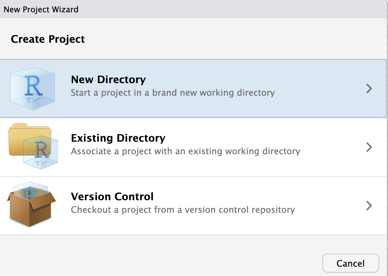
Select “New Project” from the dropdown menu. Then, click “New Directory” in the pop-up window that opens.

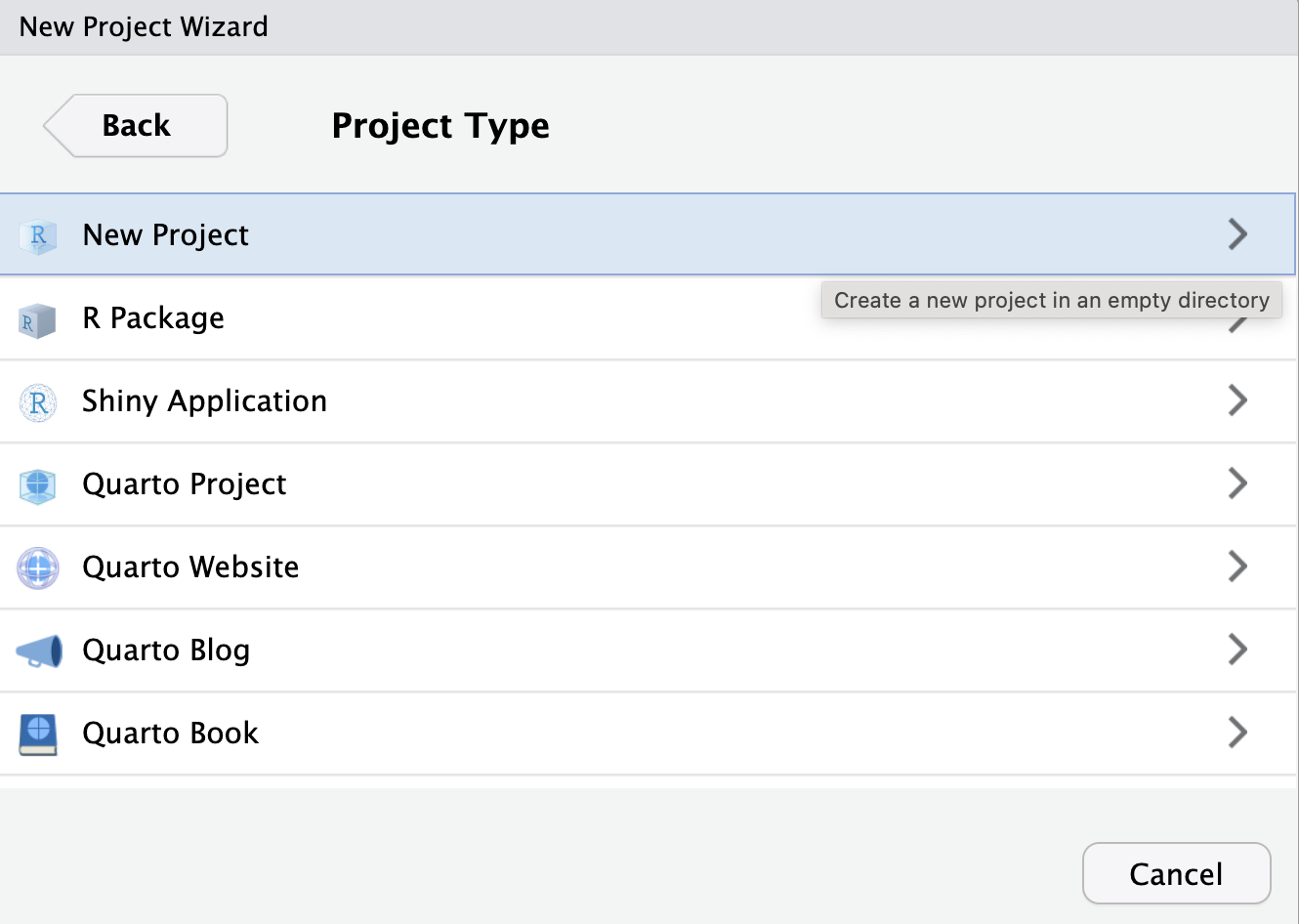
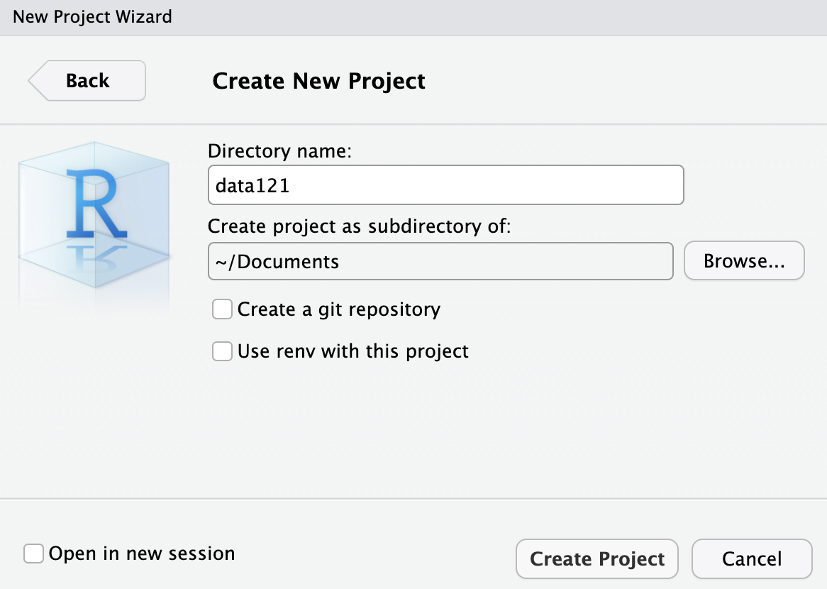
Click “New Project.” A window will appear with two fields. In the first, “Directory name:”, put data121. For the second, click the button to the right that says “Browse.”

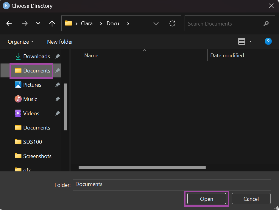
In the pop-up window that appears, navigate to your Documents folder, then select it and click “Open.” This will fill out the second field in the pop-up window. Ensure that both fields are correct, then click “Create Project.”

Warning: I strongly recommend that you not place your Project in any of the following places:

Your Downloads folder
Your Desktop
A temporary (i.e., “temp”) folder

I also recommend that you not place your Project in a cloud-based storage location (e.g., your OneDrive, Google Drive, or your iCloud folder, etc.).

Verification

Copy and paste the code below into your R console, and press the Enter key to run the code. If your project is set up correctly, you should see a message saying “Your project is in a good place” (like the one shown in the image below).

project <- tryCatch(
  usethis:::proj_path(),
  error = function(e) {
    if (class(e)[1] == "usethis_error") {
      FALSE
    } else {
      stop(e) # rethrow package not found error!
    }
  }
)

if (!isFALSE(project)) {
  cli::cli_alert_success("Project found at: {.path {project}}. Your project is in a good place.")
} else {
  cli::cli_alert_danger(
    "No project environment detected. Make sure you:\n
     1. Create and open an R project for the course.
     2. Move your Quarto file into your project folder before rendering it
    "
  )
}

Your First Quarto Document

Quarto is a software program that can be used inside of RStudio which allows you write narrative text and R code together within the same document. A Quarto document is a bit like a Microsoft Word file or Google Doc that has an R console built right into it. This allows you to create a “final product” from all your data analysis work that contains all your R code and its output (like tables and figures) and all your written explanations. You can take this final product and share it with other people, so they can see exactly what you did, and understand what your results mean.

Now, it’s time for you to open and render your very first Quarto document! You’ll be using Quarto documents to complete your lab work throughout this course, so we’ll start getting used to the workflow of rendering and turning in your final products.

Instructions for Completing the Lab and Submitting on Brightspace

Download this Quarto file
Open your computer’s file explorer, and navigate to your Downloads folder. Locate the getting_started_setup.qmd file you downloaded, and move it from your Downloads folder to your course RStudio project folder.
Double-click on the getting_started_setup.qmd file to open it in RStudio.
Add your name to the top of the Quarto document. Note: the assignment name is already included. Going forward, always add the assignment name and your name to any document that you submit on Brightspace.
Click on the button near the top middle of the editor pane.
Inspect the output in the Viewer Pane. How many checkmarks do you see? You should see eight check marks.

Finding your rendered document

Open a new window in your computer’s file explorer program (Explorer if you’re on Windows, or Finder if you’re on a Mac), and navigate to the folder where you saved your data121 RStudio Project.

In this folder you should see a filed named getting_started_setup.html. This is the output from the Quarto document you just rendered. If you double-click this file, it should open in your web browser, and you should see the same thing you saw in the RStudio Viewer pane.

Submit on Brightspace

Upload your getting_started_setup.html to the Brightspace assignment called Getting started.
Also, upload your R scripts file with all steps from the lab Step 7 saved to the Brightspace assignment.

References

SDS 100 at Smith College

Wickham, Hadley, Mara Averick, Jennifer Bryan, Winston Chang, Lucy D’Agostino McGowan, Romain François, Garrett Grolemund, et al. 2019. “Welcome to the Tidyverse.” Journal of Open Source Software 4 (43): 1686. https://doi.org/10.21105/joss.01686.

Setup

Lab instructions for Windows computers

Installing new software

Step 1: Install R

Step 2: Install RStudio

Instructions

Verification

A tour of the RStudio interface

Installing R packages

Install rstudio.prefs and customize your RStudio

Instructions

Verification

Install the course packages

Instructions

Verification

Check that rmarkdown is ready

Verification

Install dsbox

Instructions

Verification

Create a project environment for the course

Instructions

Verification

Your First Quarto Document

Instructions for Completing the Lab and Submitting on Brightspace

Finding your rendered document

Submit on Brightspace

References

Install `rstudio.prefs` and customize your RStudio

Check that `rmarkdown` is ready

Install `dsbox`