
Joining tables using two keys
Joins with the ecotourism package
First, you will work through an example using the manta_rays data set from the ecotourism package. Then, explore the ecotourism package using the help pane in RStudio and complete the same steps with another data set within the package.
In this activity, you will review and apply:
count()case_when()And joins
How to use this page:
In Part 1, the solution code is not automatically displayed, but you can see it by clicking the
Codebuttons. This gives you the opportunity to think first about how something should be done and then check to see what code was actually used. I strongly recommend you take the time to attempt an answer the question before revealing the solution.Part 2 gives you a chance to apply what you’ve learned without example solutions.
Part 1: Manta Ray sightings and ecotourism activity
In Part 1 you will analyze occurrence data for manta rays in Australia, using records from the Atlas of Living Australia (ALA). manta rays are a sensitive aquatic species whose presence may correspond with seasonal weather conditions. You will integrate sightings of manta rays with weather and seasonality (represented by annual quarter).
Data from the ecotourism library:
manta_rays: This dataset contains occurrence records for the reef manta ray observed in Australian waters from 2014 to 2024. Each row represents an individual sighting of a manta ray by location (weather stationws_id), at a particular date and time.weather: daily weather records for each station.
Take a moment to use the help page to learn more about each dataset. Use the help page in RStudio.
Step 1: Prepare a data frame of daily manta ray sightings
- Wrangle
manta_raysto create a new data framemanta_dailywhere each row represents the number of manta rays sighted each day at each weather station location. You will need to use thews_idanddatevariable. Your resulting data frame should have 319 observations.
Code
manta_daily <- manta_rays |>
  count(ws_id, date)

# Run the object name manta_daily in the console to see the result
Step 2: Connect weather conditions with manta ray sightings
- Create a new data frame called
manta_weatherthat retains all observations frommanta_dailyand adds the corresponding month and average wind speed information fromweather, maintaining the weather station-date observational unit (each row represents a weather station on a particular date). - Recall that in
DATA 121we covered joins here.
Code
manta_weather <- manta_daily |>
  left_join(weather,
            by = c("ws_id", "date")) %>%
  select(ws_id, date, n, month, wind_speed)

# Run the object name manta_weather in the console to see the result
Step 3 Create a new variable
- Create a new data frame
to_plotthat with a new variablequarter, which reflects the annual quarter time frame.
Code
to_plot <- manta_weather %>%
  mutate(quarter = case_when(
       month %in% 1:3 ~ "1",
       month %in% 4:6 ~ "2",
       month %in% 7:9 ~ "3",
       month %in% 10:12 ~ "4",
       TRUE ~ NA
     ),
     quarter = fct_relevel(quarter,
                           "1","2","3","4")) %>%
  select(ws_id, n, quarter, wind_speed) # Select to keep only the variables of interest
Step 4 Plot the relationship between weather, season, and manta ray sightings
Replicate the plot below: Create a plot that shows the relationship between daily manta ray observations and average wind speed. Color the points in the plot by the annual quarter.
- In a sentence or two, provide an interpretation of the visualization. What can we learn from this chart about the relationship between wind speed, season, and manta ray sightings?
- Recall that in
DATA 121we covered effective visualization techniques here.
Code
to_plot %>%
  drop_na(quarter) %>%
  ggplot(aes(wind_speed, n, color = quarter)) +
  geom_point(alpha = 0.8) +
  labs(
    title = "Manta Ray Count vs. Wind Speed",
    subtitle = "Colored by Annual Quarter",
    x = "Average wind speed (m/s)",
    y = "manta ray Count",
    color = "Quarter"
  ) +
  theme_minimal()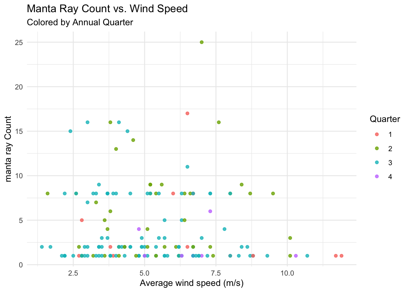
Part 2
Explore the R help page information about the ecotourism package.
- Apply the same steps you completed above to one of the other organism-specific datasets in the
ecotourismpackage.- For results that are closest to what you saw with the
manta_raydataset, I suggest using thegouldian_finchdata table and the precipitation variableprcpfrom theweatherdataset.
- For results that are closest to what you saw with the
Code
# Your code hereSubmit on Brightspace
Submit a Quarto with your work for Part 2 of the activity.