Data wrangling practice for modeling
Wrangling bike rental data for modeling
Bike sharing systems are new generation of traditional bike rentals where whole process from membership, rental and return back has become automatic. Through these systems, user is able to easily rent a bike from a particular position and return back at another position. Currently, there are about over 500 bike-sharing programs around the world which is composed of over 500 thousands bicycles. Today, there exists great interest in these systems due to their important role in traffic, environmental and health issues.
Apart from interesting real world applications of bike sharing systems, the characteristics of data being generated by these systems make them attractive for the research. Opposed to other transport services such as bus or subway, the duration of travel, departure and arrival position is explicitly recorded in these systems. This feature turns bike sharing system into a virtual sensor network that can be used for sensing mobility in the city. Hence, it is expected that most of important events in the city could be detected via monitoring these data.
Data
The data can be found in the dsbox package, and it’s called dcbikeshare. Since the dataset is distributed with the package, we don’t need to load it separately; it becomes available to us when we load the package. You can find out more about the dataset by inspecting its documentation, which you can access by running ?dcbikeshare in the Console or using the Help menu in RStudio to search for dcbikeshare.
The data include daily bike rental counts (by members and casual users) of Capital Bikeshare in Washington, DC in 2011 and 2012 as well as weather information on these days. The original data sources are http://capitalbikeshare.com/system-data and http://www.freemeteo.com.
Load the tidyverse and dsbox packages.
Step 1
Recode the season variable to be a factor with meaningful level names as outlined in the codebook, with spring as the baseline level.
Step 2
Recode the binary variables holiday and workingday to be factors with levels no (0) and yes (1), with no as the baseline level.
Step 3
Recode the yr variable to be a factor with levels 2011 and 2012, with 2011 as the baseline level.
Step 4
Recode the weathersit variable as 1 - clear, 2 - mist, 3 - light precipitation, and 4 - heavy precipitation, with clear as the baseline.
Step 5
Calculate raw temperature, feeling temperature, humidity, and windspeed as their values given in the dataset multiplied by the maximum raw values stated in the codebook for each variable. Instead of writing over the existing variables, create new ones with concise but informative names.
Step 6
Check that the sum of casual and registered adds up to cnt for each record. Hint: One way of doing this is to create a new column that takes on the value TRUE if they add up and FALSE if not, and then checking if all values in that column are TRUEs. But this is only one way, you might come up with another.
Exploratory data analysis
Step 7
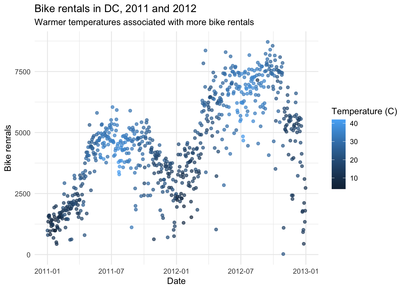
Recreate the following visualization, and interpret it in context of the data. Hint: You will need to use one of the variables you created above. The temperature plotted is the feeling temperature.
Step 8
Create a visualization displaying the relationship between bike rentals and season. Interpret the plot in context of the data.
Modeling
Step 9
Fit a linear model predicting total daily bike rentals from raw daily temperature (the version from Step 5 above), season, holiday, yr, and weather situation. Write the linear model, interpret the slope and the intercept in context of the data.