Scientific studies, confounding variables, Simpson’s Paradox

Intro to Data Analytics

Scientific Study

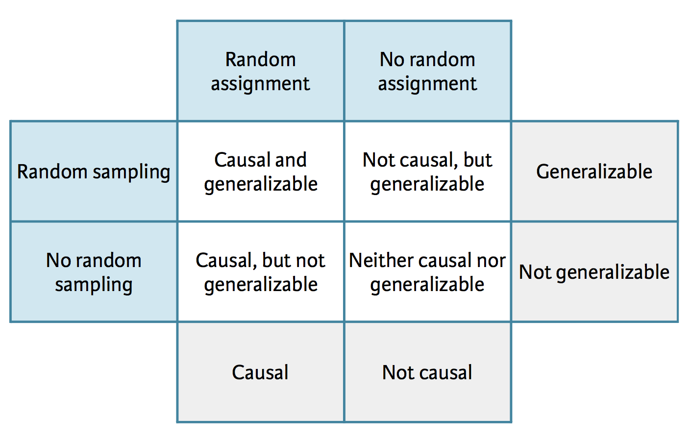
Three umbrella methodological “worlds”

Quantitative
Qualitative
Mixed

Scientific Study

Three umbrella methodological “worlds”

Quantitative – 2 of the general approaches
- Observational
- Experimental
Qualitative
Mixed

Scientific Study

Observational
- Data collection without interference (observe)
- Establish associations
Experimental
- Randomly assign subjects to treatments
- Establish causal connections

Scientific Study

Across all the modes, same key variable types:

Explanatory/independent/predictor (x)
Response/dependent/target (y)
Notation: Explanatory ~ Response
- x ~ y
- y = f(x)

Scientific Study

x –> y (direct)

x –> z –> y (mediator)

x and y both influenced by z (confounding)

Studies and conclusions

Case study: Climate change survey

Survey question

A July 2019 YouGov survey asked 1,633 GB and 1,333 USA randomly selected adults which of the following statements about the global environment best describes their view:

The climate is changing and human activity is mainly responsible

The climate is changing and human activity is partly responsible, together with other factors

The climate is changing but human activity is not responsible at all

The climate is not changing

Survey data

	The climate is changing and human activity is mainly responsible	The climate is changing and human activity is partly responsible, together with other factors	The climate is changing but human activity is not responsible at all	The climate is not changing	Don't know	Sum
GB	833	604	49	33	114	1633
US	507	493	120	80	133	1333
Sum	1340	1097	169	113	247	2966

Source: YouGov - International Climate Change Survey

Question

What percent of all respondents think the climate is changing and
human activity is mainly responsible?

	The climate is changing and human activity is mainly responsible	The climate is changing and human activity is partly responsible, together with other factors	The climate is changing but human activity is not responsible at all	The climate is not changing	Don't know	Sum
GB	833	604	49	33	114	1633
US	507	493	120	80	133	1333
Sum	1340	1097	169	113	247	2966

(all <- 1340 / 2966)

[1] 0.4517869

Question

What percent of all respondents think the climate is changing and
human activity is mainly responsible?

	The climate is changing and human activity is mainly responsible	The climate is changing and human activity is partly responsible, together with other factors	The climate is changing but human activity is not responsible at all	The climate is not changing	Don't know	Sum
GB	833	604	49	33	114	1633
US	507	493	120	80	133	1333
Sum	1340	1097	169	113	247	2966

Probability

P(A) –> P(Human Activity) = 45%

Question

What percent of GB respondents think the climate is changing and
human activity is mainly responsible?

	The climate is changing and human activity is mainly responsible	The climate is changing and human activity is partly responsible, together with other factors	The climate is changing but human activity is not responsible at all	The climate is not changing	Don't know	Sum
GB	833	604	49	33	114	1633
US	507	493	120	80	133	1333
Sum	1340	1097	169	113	247	2966

(gb <- 833 / 1633)

[1] 0.5101041

P(A|B) Conditional probability –> P(Human Activity | GB) = 51%

Question

What percent of US respondents think the climate is changing and
human activity is mainly responsible?

	The climate is changing and human activity is mainly responsible	The climate is changing and human activity is partly responsible, together with other factors	The climate is changing but human activity is not responsible at all	The climate is not changing	Don't know	Sum
GB	833	604	49	33	114	1633
US	507	493	120	80	133	1333
Sum	1340	1097	169	113	247	2966

(us <- 507 / 1333)

[1] 0.3803451

P(A|B) Conditional probability –> P(Human Activity | US) = 38%

Based on the percentages we calculated, does there appear to be a relationship between country and beliefs about climate change? If yes, could there be another variable that explains this relationship?

all

[1] 0.4517869

gb

[1] 0.5101041

us

[1] 0.3803451

Conditional probability

Notation: \(P(A | B)\): Probability of event A given event B

What is the probability that it will be unseasonably warm tomorrow?
What is the probability that it will be unseasonably warm tomorrow, given that it was unseasonably warm today?

Independence

We want to determine whether knowing A happened tells you something about B, or vice versa – in which case they are not independent.
If not, they are said to be independent
\(P(A | B) = P(A)\) the probability of event A given event B
If knowing B doesn’t change anything about the probability of A then they are independent.

Is there independence in our climate change example?

Simpson’s Paradox (using Berkeley admissions data)

Berkeley admissions data

Study carried out by the Graduate Division of the University of California, Berkeley in the early 1970’s to evaluate whether there was a gender bias in graduate admissions.
Data from six departments (we’ll call them A-F)
Information on whether the applicant was male or female and whether they were admitted or rejected.
First, evaluate whether the percentage of males admitted is indeed higher than females, overall. Next,calculate the same percentage for each department.
Using the dataset ucbadmit from the dsbox package

Data

# A tibble: 4,526 × 3
   admit    gender dept 
   <fct>    <fct>  <ord>
 1 Admitted Male   A    
 2 Admitted Male   A    
 3 Admitted Male   A    
 4 Admitted Male   A    
 5 Admitted Male   A    
 6 Admitted Male   A    
 7 Admitted Male   A    
 8 Admitted Male   A    
 9 Admitted Male   A    
10 Admitted Male   A    
11 Admitted Male   A    
12 Admitted Male   A    
13 Admitted Male   A    
14 Admitted Male   A    
15 Admitted Male   A    
# ℹ 4,511 more rows

# A tibble: 2 × 2
  gender     n
  <fct>  <int>
1 Female  1835
2 Male    2691

# A tibble: 6 × 2
  dept      n
  <ord> <int>
1 A       933
2 B       585
3 C       918
4 D       792
5 E       584
6 F       714

# A tibble: 2 × 2
  admit        n
  <fct>    <int>
1 Rejected  2771
2 Admitted  1755

What function did I use to create the tables on the right?

ucbadmit %>%
  count(gender)
ucbadmit %>%
  count(dept)
ucbadmit %>%
  count(admit)

We want to answer two questions:

If an applicant is male, what’s the probability he was admitted?
If an applicant is female, what’s the probability she was admitted?

We can do this by using count() and specifying gender and admit as the variables of interest, giving us the frequencies we need.

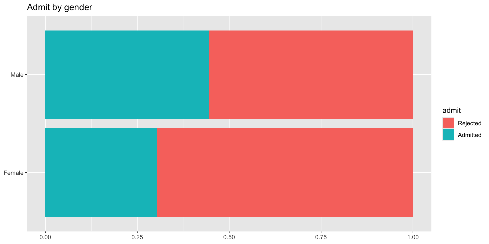
What can you say about overall gender distribution?

Hint: Calculate the following probabilities: \(P(Admit | Male)\) and \(P(Admit | Female)\).

ucbadmit %>%
  count(gender, admit)

# A tibble: 4 × 3
  gender admit        n
  <fct>  <fct>    <int>
1 Female Rejected  1278
2 Female Admitted   557
3 Male   Rejected  1493
4 Male   Admitted  1198

ucbadmit %>%
  count(gender, admit) %>%
  group_by(gender) %>%
  mutate(prop_admit = n / sum(n))

# A tibble: 4 × 4
# Groups:   gender [2]
  gender admit        n prop_admit
  <fct>  <fct>    <int>      <dbl>
1 Female Rejected  1278      0.696
2 Female Admitted   557      0.304
3 Male   Rejected  1493      0.555
4 Male   Admitted  1198      0.445

\(P(Admit | Female)\) = 0.304
\(P(Admit | Male)\) = 0.445

We can group our counts by gender which will separate them into two groups. Then for each group calculate the proportion admitted by taking the sum(n) for the group—the total n women separate from the total n men—and dividing the number admitted by the total for that group.

ggplot(ucbadmit, aes(y = gender, fill = admit)) +
  geom_bar(position = "fill") + 
  labs(title = "Admit by gender",
       y = NULL, x = NULL)

Gender distribution by department?

ucbadmit %>%
  count(dept, gender, admit)

# A tibble: 24 × 4
   dept  gender admit        n
   <ord> <fct>  <fct>    <int>
 1 A     Female Rejected    19
 2 A     Female Admitted    89
 3 A     Male   Rejected   313
 4 A     Male   Admitted   512
 5 B     Female Rejected     8
 6 B     Female Admitted    17
 7 B     Male   Rejected   207
 8 B     Male   Admitted   353
 9 C     Female Rejected   391
10 C     Female Admitted   202
# ℹ 14 more rows

How can we wrangle this table to make it easier to see the rejected/admitted women and men for each department?

Gender distribution by department?

ucbadmit %>%
  count(dept, gender, admit) %>%
  pivot_wider(names_from = dept, values_from = n)

# A tibble: 4 × 8
  gender admit        A     B     C     D     E     F
  <fct>  <fct>    <int> <int> <int> <int> <int> <int>
1 Female Rejected    19     8   391   244   299   317
2 Female Admitted    89    17   202   131    94    24
3 Male   Rejected   313   207   205   279   138   351
4 Male   Admitted   512   353   120   138    53    22

Gender distribution, by department

Plot
Code

ggplot(ucbadmit, aes(y = gender, fill = admit)) +
  geom_bar(position = "fill") +
  facet_wrap(. ~ dept) +
  scale_x_continuous(labels = label_percent()) +
  labs(title = "Admissions by gender and department",
       x = NULL, y = NULL, fill = NULL) +
  theme(legend.position = "bottom")

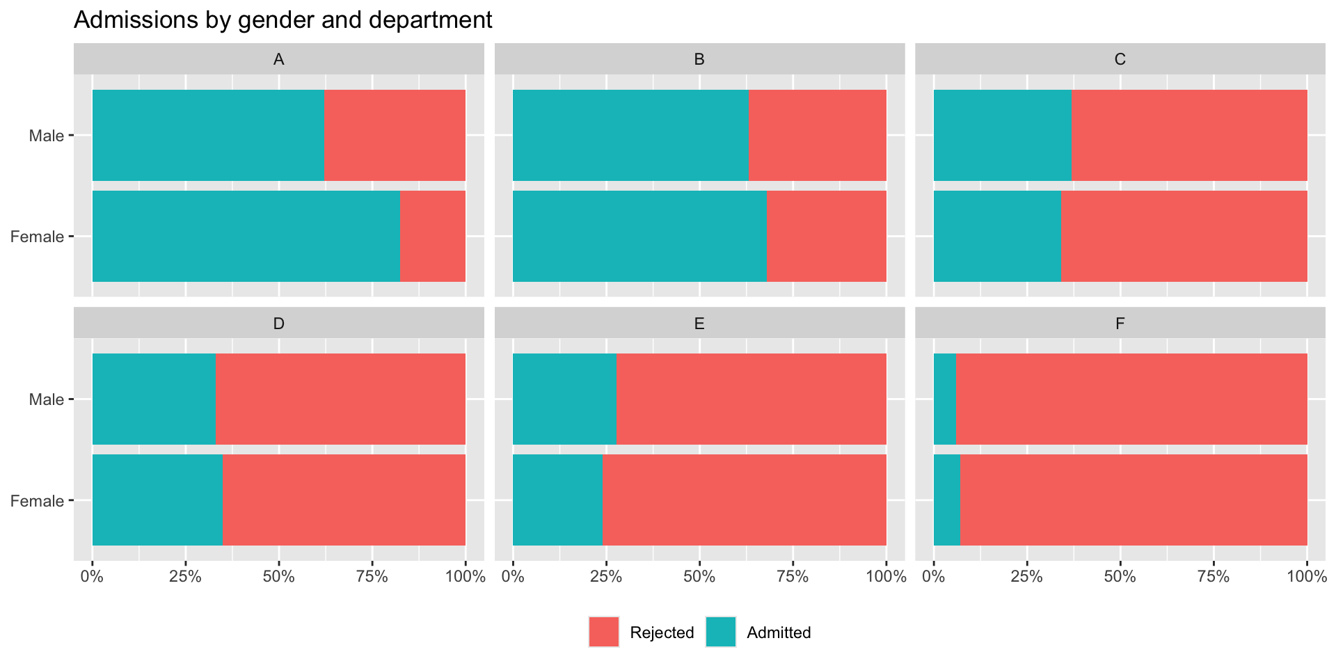
Case for gender discrimination?

When we look at our two pictures side by side they seem to be telling us a different story.

Let’s take a closer look at the departments

For each dept., we’ll compute the proportion of men and women who were admitted.

ucbadmit %>%
  count(dept, gender, admit) %>%
  group_by(dept, gender) %>%
  mutate(
    n_applied  = sum(n),
    prop_admit = n / n_applied
    )

# A tibble: 24 × 6
# Groups:   dept, gender [12]
   dept  gender admit        n n_applied prop_admit
   <ord> <fct>  <fct>    <int>     <int>      <dbl>
 1 A     Female Rejected    19       108      0.176
 2 A     Female Admitted    89       108      0.824
 3 A     Male   Rejected   313       825      0.379
 4 A     Male   Admitted   512       825      0.621
 5 B     Female Rejected     8        25      0.32 
 6 B     Female Admitted    17        25      0.68 
 7 B     Male   Rejected   207       560      0.370
 8 B     Male   Admitted   353       560      0.630
 9 C     Female Rejected   391       593      0.659
10 C     Female Admitted   202       593      0.341
# ℹ 14 more rows

Closer look at departments

Output
Code

# A tibble: 12 × 5
# Groups:   dept, gender [12]
   dept  gender n_admitted n_applied prop_admit
   <ord> <fct>       <int>     <int>      <dbl>
 1 A     Female         89       108     0.824 
 2 A     Male          512       825     0.621 
 3 B     Female         17        25     0.68  
 4 B     Male          353       560     0.630 
 5 C     Female        202       593     0.341 
 6 C     Male          120       325     0.369 
 7 D     Female        131       375     0.349 
 8 D     Male          138       417     0.331 
 9 E     Female         94       393     0.239 
10 E     Male           53       191     0.277 
11 F     Female         24       341     0.0704
12 F     Male           22       373     0.0590

ucbadmit %>%
  count(dept, gender, admit) %>%
  group_by(dept, gender) %>%
  mutate(
    n_applied  = sum(n),
    prop_admit = n / n_applied
    ) %>%
  filter(admit == "Admitted") %>% # Filter becuase we only need the proportion admitted
  rename(n_admitted = n) %>%
  select(-admit) # Select all columns except for admit

What do we know now?

In dept A:
- 108 women applied and 89 were admitted.
- 825 men applied and 512 were admitted.
So even though a high proportion of women were admitted, a much smaller number applied which means that there is still a gender issue in terms of who is attracted to the field.
So there isn’t necessarily gender discrimination in admissions in dept A, but there is an issue in terms of the distribution of who applies.

Consider dept F, the number of applications is pretty similar for both genders, the number admitted is similar, the proportion of women admitted is higher.

What can we conclude? It is the case that gender discrimination is a concern, but depending on what question you are asking and whether or not you consider the third variable of department, the conclusions you arrive at could be different.

Simpson’s paradox

Relationship between two variables

# A tibble: 8 × 3
      x     y z    
  <dbl> <dbl> <chr>
1     2     4 A    
2     3     3 A    
3     4     2 A    
4     5     1 A    
5     6    11 B    
6     7    10 B    
7     8     9 B    
8     9     8 B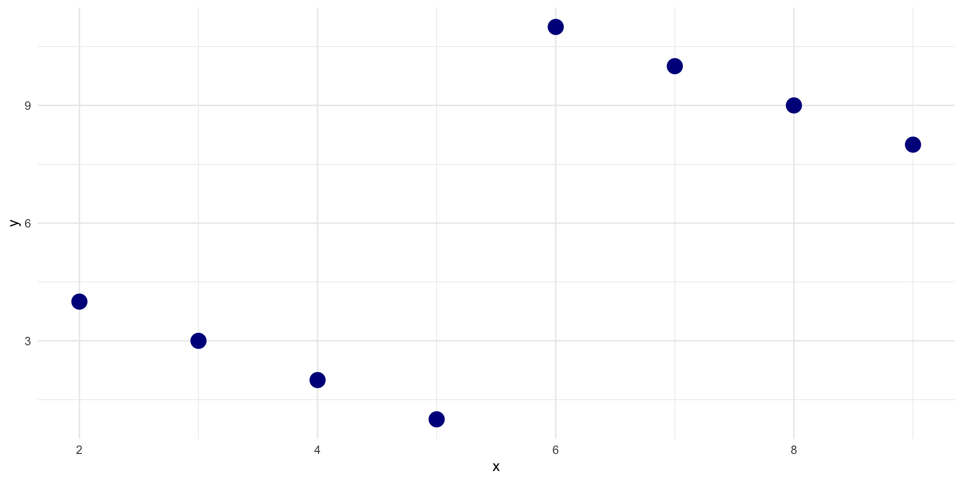

Relationship between two variables

# A tibble: 8 × 3
      x     y z    
  <dbl> <dbl> <chr>
1     2     4 A    
2     3     3 A    
3     4     2 A    
4     5     1 A    
5     6    11 B    
6     7    10 B    
7     8     9 B    
8     9     8 B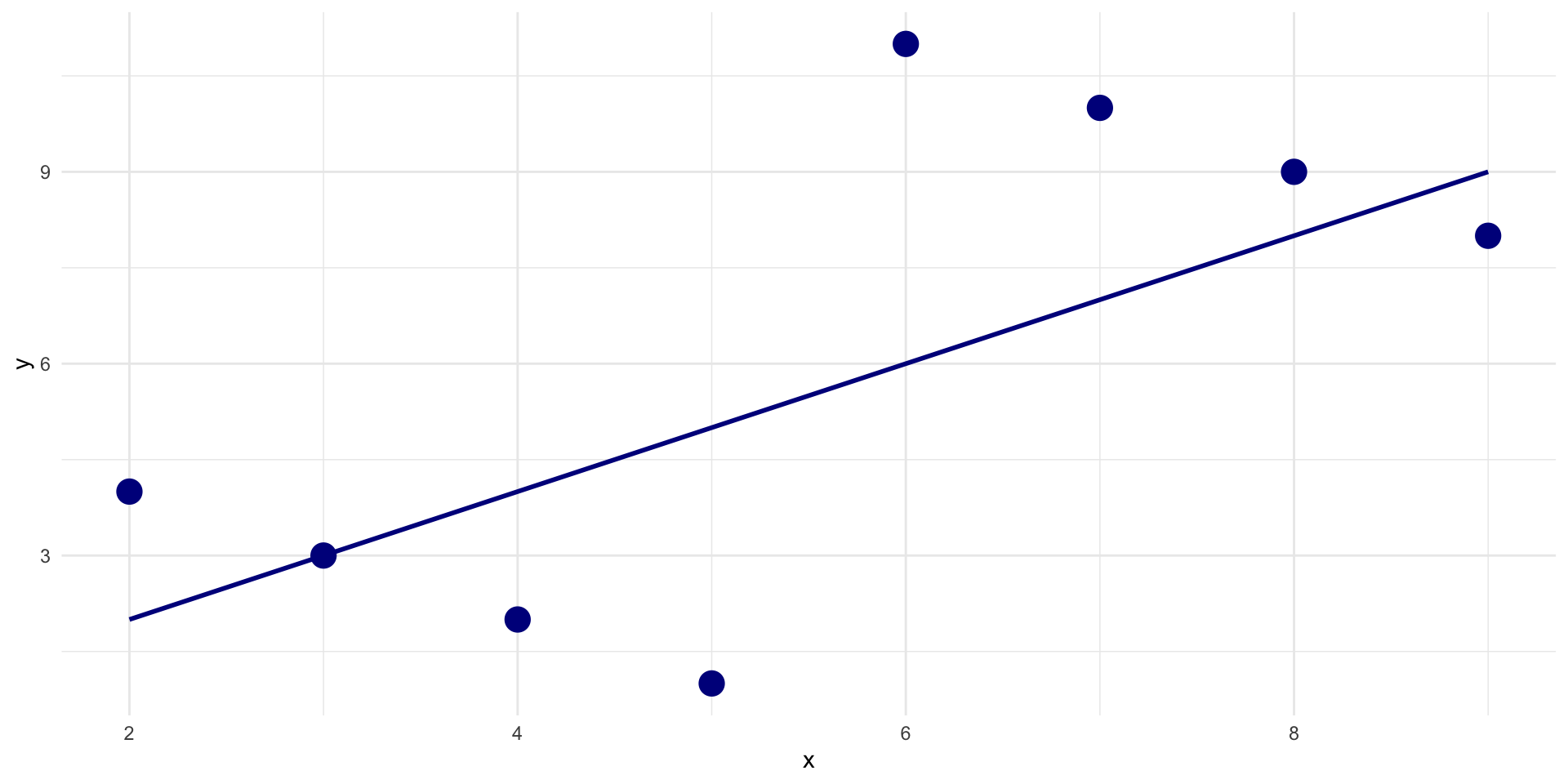

Considering a third variable

# A tibble: 8 × 3
      x     y z    
  <dbl> <dbl> <chr>
1     2     4 A    
2     3     3 A    
3     4     2 A    
4     5     1 A    
5     6    11 B    
6     7    10 B    
7     8     9 B    
8     9     8 B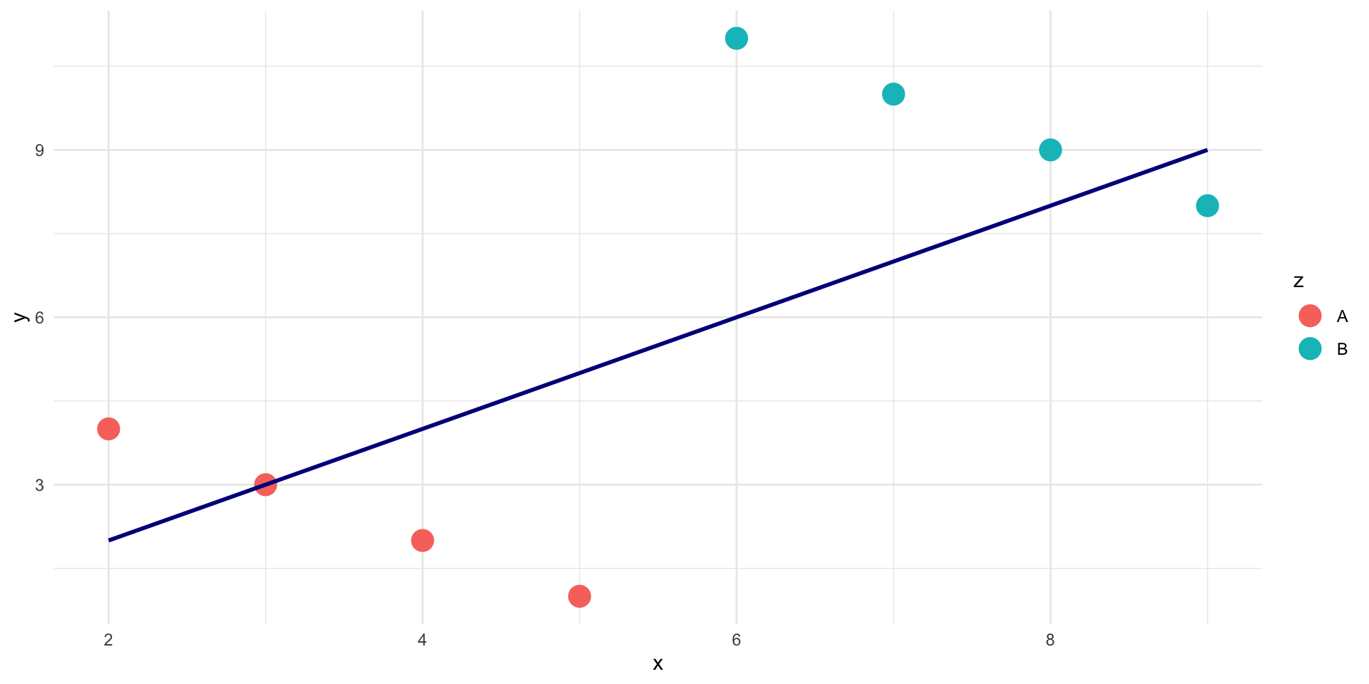

Relationship between three variables

# A tibble: 8 × 3
      x     y z    
  <dbl> <dbl> <chr>
1     2     4 A    
2     3     3 A    
3     4     2 A    
4     5     1 A    
5     6    11 B    
6     7    10 B    
7     8     9 B    
8     9     8 B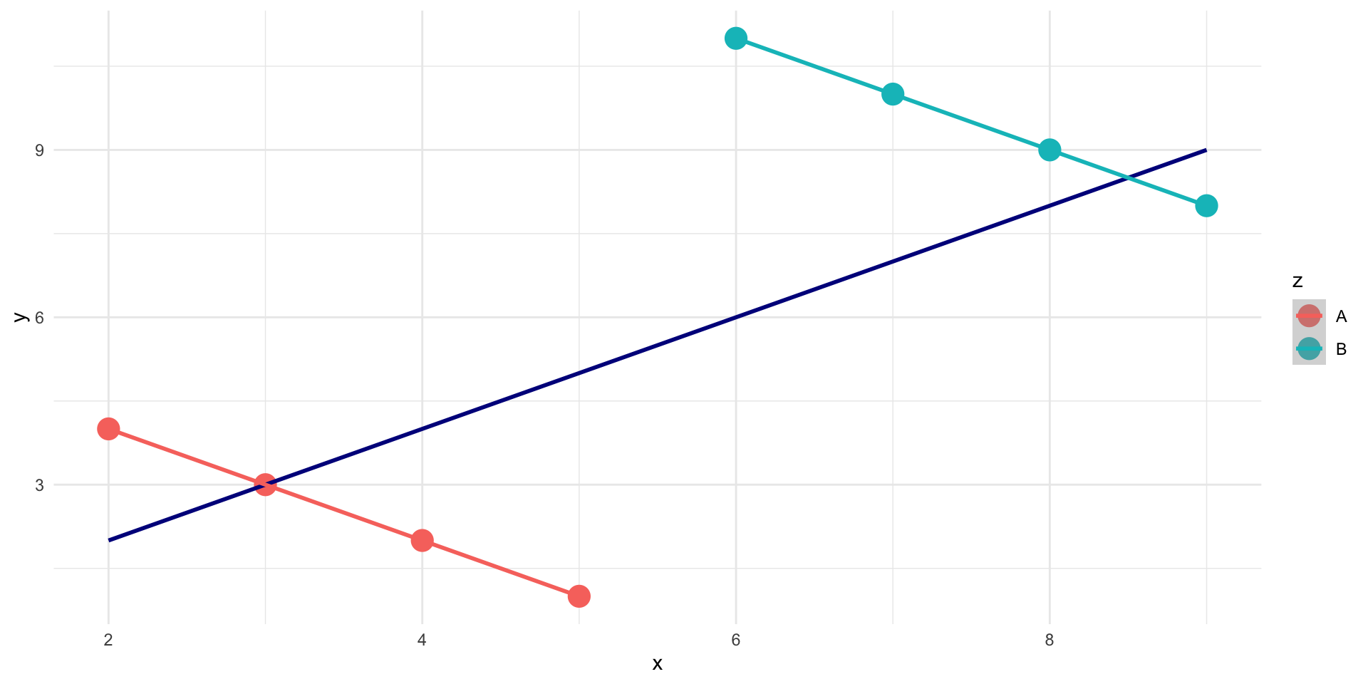

Simpson’s paradox

Not considering an important variable when studying a relationship can result in Simpson’s paradox
Simpson’s paradox illustrates
- omission of an explanatory variable can affect the measure of association between another explanatory variable and a response variable
Inclusion of a third variable in the analysis can change the apparent relationship between the other two variables

Review at home: `group_by()` and `count()`

What does group_by() do?

group_by() takes an existing data frame and converts it into a grouped data frame where subsequent operations are performed “once per group”

ucbadmit

# A tibble: 4,526 × 3
   admit    gender dept 
   <fct>    <fct>  <ord>
 1 Admitted Male   A    
 2 Admitted Male   A    
 3 Admitted Male   A    
 4 Admitted Male   A    
 5 Admitted Male   A    
 6 Admitted Male   A    
 7 Admitted Male   A    
 8 Admitted Male   A    
 9 Admitted Male   A    
10 Admitted Male   A    
# ℹ 4,516 more rows

ucbadmit %>% 
  group_by(gender)

# A tibble: 4,526 × 3
# Groups:   gender [2]
   admit    gender dept 
   <fct>    <fct>  <ord>
 1 Admitted Male   A    
 2 Admitted Male   A    
 3 Admitted Male   A    
 4 Admitted Male   A    
 5 Admitted Male   A    
 6 Admitted Male   A    
 7 Admitted Male   A    
 8 Admitted Male   A    
 9 Admitted Male   A    
10 Admitted Male   A    
# ℹ 4,516 more rows

What does group_by() not do?

group_by() does not sort the data, arrange() does

ucbadmit %>% 
  group_by(gender)

# A tibble: 4,526 × 3
# Groups:   gender [2]
   admit    gender dept 
   <fct>    <fct>  <ord>
 1 Admitted Male   A    
 2 Admitted Male   A    
 3 Admitted Male   A    
 4 Admitted Male   A    
 5 Admitted Male   A    
 6 Admitted Male   A    
 7 Admitted Male   A    
 8 Admitted Male   A    
 9 Admitted Male   A    
10 Admitted Male   A    
# ℹ 4,516 more rows

ucbadmit %>% 
  arrange(gender)

# A tibble: 4,526 × 3
   admit    gender dept 
   <fct>    <fct>  <ord>
 1 Admitted Female A    
 2 Admitted Female A    
 3 Admitted Female A    
 4 Admitted Female A    
 5 Admitted Female A    
 6 Admitted Female A    
 7 Admitted Female A    
 8 Admitted Female A    
 9 Admitted Female A    
10 Admitted Female A    
# ℹ 4,516 more rows

What does group_by() not do?

group_by() does not create frequency tables, count() does

ucbadmit %>% 
  group_by(gender)

# A tibble: 4,526 × 3
# Groups:   gender [2]
   admit    gender dept 
   <fct>    <fct>  <ord>
 1 Admitted Male   A    
 2 Admitted Male   A    
 3 Admitted Male   A    
 4 Admitted Male   A    
 5 Admitted Male   A    
 6 Admitted Male   A    
 7 Admitted Male   A    
 8 Admitted Male   A    
 9 Admitted Male   A    
10 Admitted Male   A    
# ℹ 4,516 more rows

ucbadmit %>% 
  count(gender)

# A tibble: 2 × 2
  gender     n
  <fct>  <int>
1 Female  1835
2 Male    2691

Undo grouping with ungroup()

ucbadmit %>%
  count(gender, admit) %>%
  group_by(gender) %>%
  mutate(prop_admit = n / sum(n)) %>%
  select(gender, prop_admit)

# A tibble: 4 × 2
# Groups:   gender [2]
  gender prop_admit
  <fct>       <dbl>
1 Female      0.696
2 Female      0.304
3 Male        0.555
4 Male        0.445

ucbadmit %>%
  count(gender, admit) %>%
  group_by(gender) %>%
  mutate(prop_admit = n / sum(n)) %>%
  select(gender, prop_admit) %>%
  ungroup()

# A tibble: 4 × 2
  gender prop_admit
  <fct>       <dbl>
1 Female      0.696
2 Female      0.304
3 Male        0.555
4 Male        0.445

count() is a short-hand

count() is a short-hand for group_by() and then summarize() to count the number of observations in each group

ucbadmit %>%
  group_by(gender) %>%
  summarize(n = n())

# A tibble: 2 × 2
  gender     n
  <fct>  <int>
1 Female  1835
2 Male    2691

ucbadmit %>%
  count(gender)

# A tibble: 2 × 2
  gender     n
  <fct>  <int>
1 Female  1835
2 Male    2691

count can take multiple arguments

ucbadmit %>%
  group_by(gender, admit) %>%
  summarize(n = n())

# A tibble: 4 × 3
# Groups:   gender [2]
  gender admit        n
  <fct>  <fct>    <int>
1 Female Rejected  1278
2 Female Admitted   557
3 Male   Rejected  1493
4 Male   Admitted  1198

ucbadmit %>%
  count(gender, admit)

# A tibble: 4 × 3
  gender admit        n
  <fct>  <fct>    <int>
1 Female Rejected  1278
2 Female Admitted   557
3 Male   Rejected  1493
4 Male   Admitted  1198

`summarize()` after `group_by()`

count() ungroups after itself
summarize() peels off one layer of grouping by default, or you can specify a different behavior

ucbadmit %>%
  group_by(gender, admit) %>%
  summarize(n = n())

`summarise()` has grouped output by 'gender'. You can override using the
`.groups` argument.

# A tibble: 4 × 3
# Groups:   gender [2]
  gender admit        n
  <fct>  <fct>    <int>
1 Female Rejected  1278
2 Female Admitted   557
3 Male   Rejected  1493
4 Male   Admitted  1198

Scientific studies, confounding variables, Simpson’s Paradox

Scientific Study

Scientific Study

Scientific Study

Scientific Study

Scientific Study

Studies and conclusions

Case study: Climate change survey

Survey question

Survey data

Question

Question

Question

Question

Conditional probability

Independence

Simpson’s Paradox (using Berkeley admissions data)

Berkeley admissions data

Data

Overall gender distribution

Gender distribution by department?

Gender distribution by department?

Gender distribution, by department

Case for gender discrimination?

Let’s take a closer look at the departments

Closer look at departments

What do we know now?

Simpson’s paradox

Relationship between two variables

Relationship between two variables

Considering a third variable

Relationship between three variables

Simpson’s paradox

Review at home: group_by() and count()

What does group_by() do?

What does group_by() not do?

What does group_by() not do?

Undo grouping with ungroup()

count() is a short-hand

count can take multiple arguments

summarize() after group_by()

Review at home: `group_by()` and `count()`

`summarize()` after `group_by()`