Fitting and Interpreting Models

Intro to Data Analytics

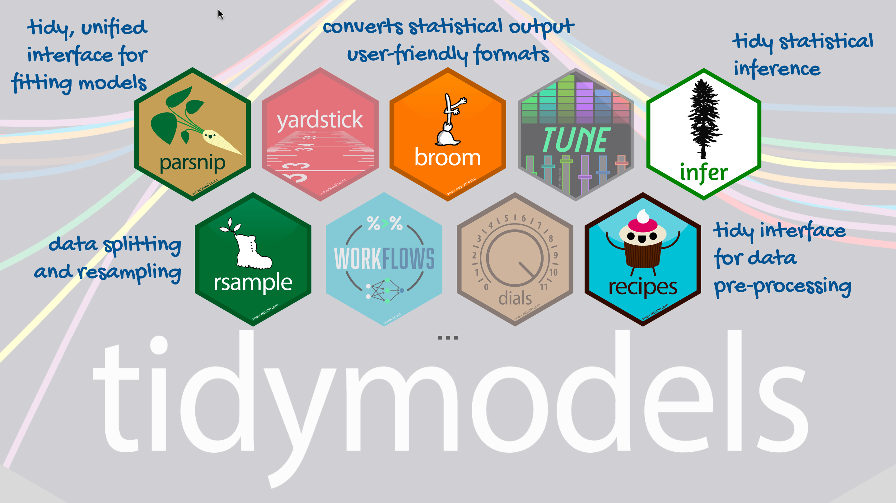
Getting started

• Install and load tidymodels (see next slide if you get thrown an error).

• Download and place the R script file LM-code.R in your working directory.

What to do if you face an error when installing and loading the tidymodels package.

• The newest version of tidymodels requires you to either:

  • Update the rlang package. Use install.packages("rlang") to update.

  • Update your version of RStudio. To do so, you will need to download the newest release of RStudio (that came out just after we started the semester):

    • https://posit.co/download/rstudio-desktop/#download

    • Note: you do not need to uninstall anything in order to update.

How do we use models?

• Explanation – Characterize relationship between y and x by using
  • slope for numerical explanatory variables
  • differences for categorical explanatory variables
• Prediction – plug in x, get predicted y

Models with numerical explanatory variables

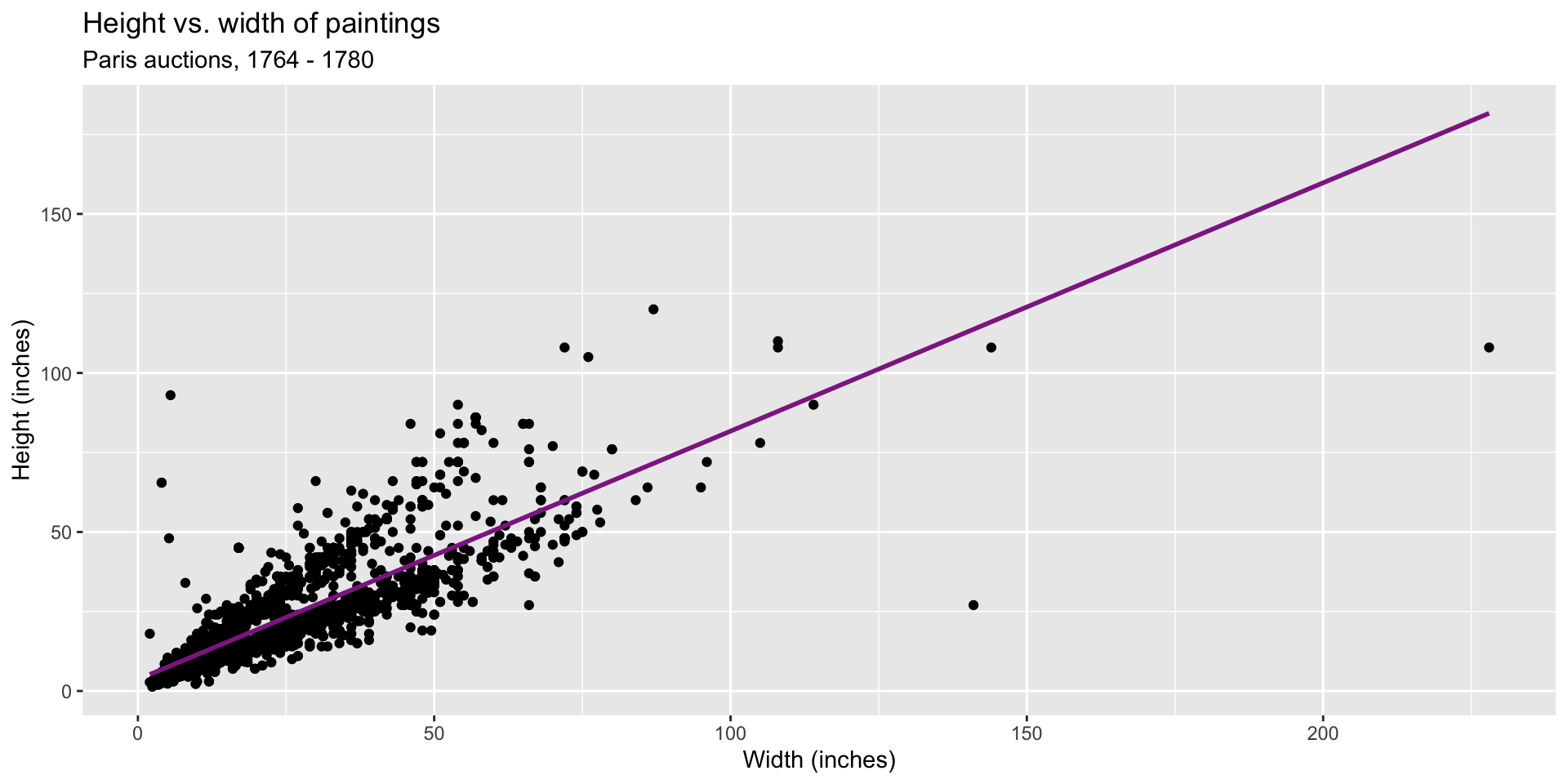
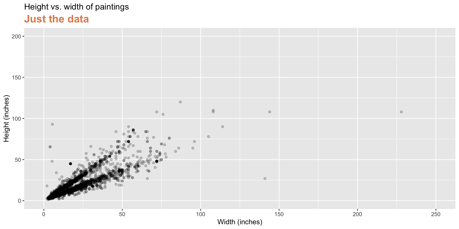
Data: Paris Paintings

• Number of observations: 3393
• Number of variables: 61

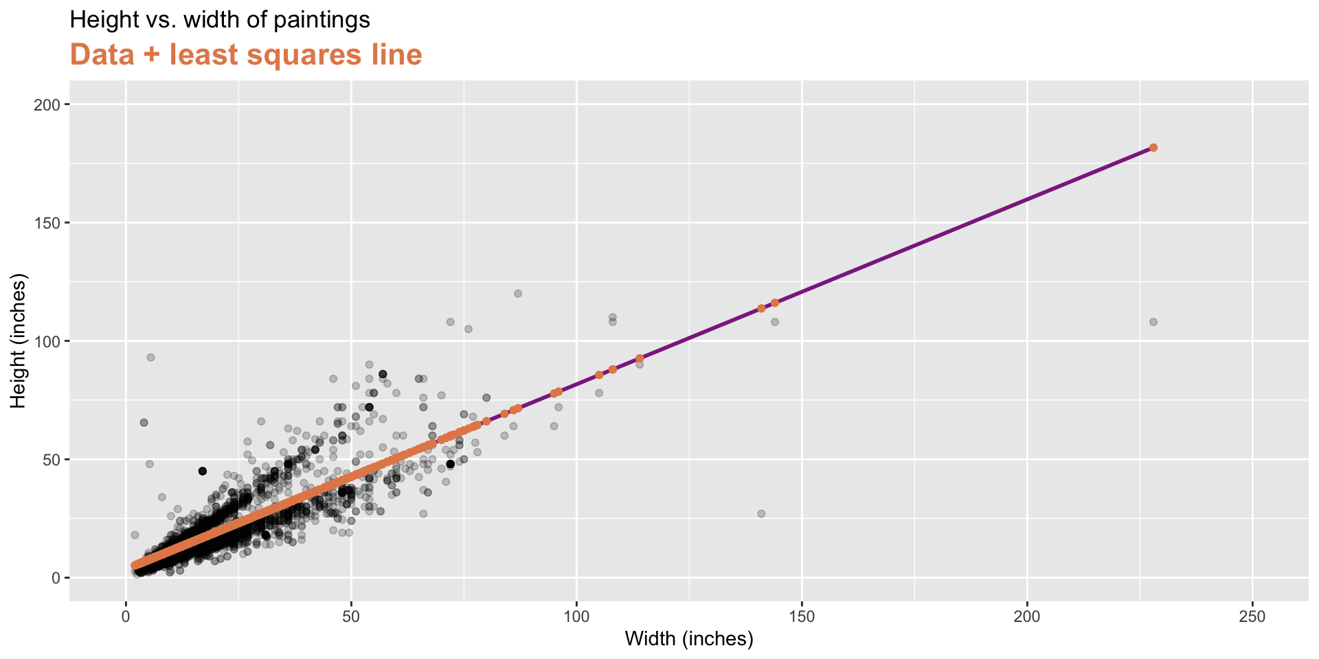
Goal: Predict height from width

\[\widehat{height}_{i} = \beta_0 + \beta_1 \times width_{i}\]

Step 1: Specify model

linear_reg()

Linear Regression Model Specification (regression)

Computational engine: lm 

Step 2: Set model fitting engine

linear_reg() %>%
  set_engine("lm") # lm: linear model

Linear Regression Model Specification (regression)

Computational engine: lm 

Step 3: Fit model & estimate parameters

… using formula syntax

linear_reg() %>%
  set_engine("lm") %>%
  fit(Height_in ~ Width_in, data = pp)

parsnip model object


Call:
stats::lm(formula = Height_in ~ Width_in, data = data)

Coefficients:
(Intercept)     Width_in  
     3.6214       0.7808  

A closer look at model output

parsnip model object


Call:
stats::lm(formula = Height_in ~ Width_in, data = data)

Coefficients:
(Intercept)     Width_in  
     3.6214       0.7808  

\[\widehat{height}_{i} = 3.6214 + 0.7808 \times width_{i}\]

A tidy look at model output

linear_reg() %>%
  set_engine("lm") %>%
  fit(Height_in ~ Width_in, data = pp) %>%
  tidy()

# A tibble: 2 × 5
  term        estimate std.error statistic  p.value
  <chr>          <dbl>     <dbl>     <dbl>    <dbl>
1 (Intercept)    3.62    0.254        14.3 8.82e-45
2 Width_in       0.781   0.00950      82.1 0       

\[\widehat{height}_{i} = 3.62 + 0.781 \times width_{i}\]

Slope and intercept

\[\widehat{height}_{i} = 3.62 + 0.781 \times width_{i}\]

• Slope: For each additional inch the painting is wider, the height is expected to be higher, on average, by 0.781 inches.

• Intercept: Paintings that are 0 inches wide are expected to be 3.62 inches high, on average. (Does this make sense?)

Your turn

• Take out your notes on regression from last week.

• If you haven’t already, download and place the LM-code.R R script file in your working directory.

• Let’s work through some examples.

Parameter estimation

Linear model with a single predictor

• We’re interested in \(\beta_0\) (population parameter for the intercept) and \(\beta_1\) (population parameter for the slope) in the following model:

\[\widehat{y}_{i} = \beta_0 + \beta_1*x_{i}\]

• Tough luck, you can’t have them…

• So we use sample statistics to estimate them:

\[\widehat{y}_{i} = b_0 + b_1*x_{i}\]

Least squares regression

• The regression line minimizes the sum of squared residuals.

• If \(e_i = y_i - \hat{y}_i\), then, the regression line minimizes \(\sum_{i = 1}^n e_i^2\).

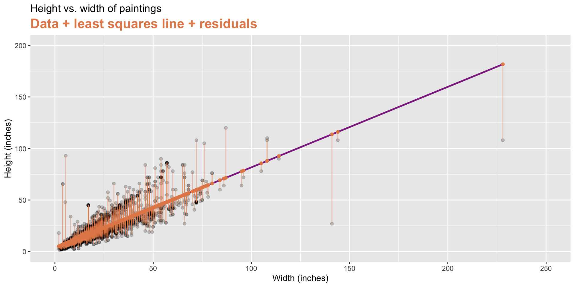
Visualizing residuals

Visualizing residuals (cont.)

Visualizing residuals (cont.)

Properties of least squares regression

• The regression line goes through the center of mass point, the coordinates corresponding to average \(x\) and average \(y\), \((\bar{x}, \bar{y})\):

\[\bar{y} = b_0 + b_1 \bar{x} ~ \rightarrow ~ b_0 = \bar{y} - b_1 \bar{x}\]

• The slope has the same sign as the correlation coefficient: \(b_1 = r \frac{s_y}{s_x}\)

• The sum of the residuals is zero: \(\sum_{i = 1}^n e_i = 0\)

• The residuals and \(x\) values are uncorrelated: As you travel along the x axis, how far your model is from the observed data doesn’t vary along with x, the residual doesn’t increase because x increases.

Models with categorical explanatory variables

Models with categorical predictors

• Up to now dependent and independent variables are continuous

• But life is not continuous

• Categorical variables have special properties in models

Categorical predictor with 2 levels

# A tibble: 3,393 × 3
   name      Height_in landsALL
   <chr>         <dbl>    <dbl>
 1 L1764-2          37        0
 2 L1764-3          18        0
 3 L1764-4          13        1
 4 L1764-5a         14        1
 5 L1764-5b         14        1
 6 L1764-6           7        0
 7 L1764-7a          6        0
 8 L1764-7b          6        0
 9 L1764-8          15        0
10 L1764-9a          9        0
11 L1764-9b          9        0
12 L1764-10a        16        1
13 L1764-10b        16        1
14 L1764-10c        16        1
15 L1764-11         20        0
16 L1764-12a        14        1
17 L1764-12b        14        1
18 L1764-13a        15        1
19 L1764-13b        15        1
20 L1764-14         37        0
# ℹ 3,373 more rows

• landsALL = 0: No landscape features
• landsALL = 1: Some landscape features

Height & landscape features

linear_reg() %>%
  set_engine("lm") %>%
  fit(Height_in ~ factor(landsALL), data = pp) %>%
  tidy()

# A tibble: 2 × 5
  term              estimate std.error statistic  p.value
  <chr>                <dbl>     <dbl>     <dbl>    <dbl>
1 (Intercept)          22.7      0.328      69.1 0       
2 factor(landsALL)1    -5.65     0.532     -10.6 7.97e-26

• Note: we use factor() because we want R to read the numerical dummy variable as two categories (not as numerical values).

Height & landscape features

\[\widehat{Height_{in}} = 22.7 - 5.645~landsALL\]

• Slope: Paintings with landscape features are expected, on average, to be 5.645 inches shorter than paintings without landscape features
  • Compares baseline level (landsALL = 0) to the other level (landsALL = 1)
• Intercept: Paintings that don’t have landscape features are expected, on average, to be 22.7 inches tall

Models with categorical predictors

Extend this out to multiple categories in one variable

• Each category coded to separate indicator (1/0) variable
• For example, relationship between height and school

linear_reg() %>%
  set_engine("lm") %>%
  fit(Height_in ~ school_pntg, data = pp) %>%
  tidy()

# A tibble: 7 × 5
  term            estimate std.error statistic p.value
  <chr>              <dbl>     <dbl>     <dbl>   <dbl>
1 (Intercept)        14.0       10.0     1.40  0.162  
2 school_pntgD/FL     2.33      10.0     0.232 0.816  
3 school_pntgF       10.2       10.0     1.02  0.309  
4 school_pntgG        1.65      11.9     0.139 0.889  
5 school_pntgI       10.3       10.0     1.02  0.306  
6 school_pntgS       30.4       11.4     2.68  0.00744
7 school_pntgX        2.87      10.3     0.279 0.780  

Dummy variables

• When the categorical explanatory variable has many levels, they’re encoded to dummy variables
• Each coefficient describes the expected difference between heights in that particular school compared to the baseline level. Note: we can specify the baseline level using the forcats package fct_relevel.

Categorical predictor with 3+ levels

school_pntg	D_FL	F	G	I	S	X
A	0	0	0	0	0	0
D/FL	1	0	0	0	0	0
F	0	1	0	0	0	0
G	0	0	1	0	0	0
I	0	0	0	1	0	0
S	0	0	0	0	1	0
X	0	0	0	0	0	1

# A tibble: 3,393 × 3
   name      Height_in school_pntg
   <chr>         <dbl> <chr>      
 1 L1764-2          37 F          
 2 L1764-3          18 I          
 3 L1764-4          13 D/FL       
 4 L1764-5a         14 F          
 5 L1764-5b         14 F          
 6 L1764-6           7 I          
 7 L1764-7a          6 F          
 8 L1764-7b          6 F          
 9 L1764-8          15 I          
10 L1764-9a          9 D/FL       
11 L1764-9b          9 D/FL       
12 L1764-10a        16 X          
13 L1764-10b        16 X          
14 L1764-10c        16 X          
15 L1764-11         20 D/FL       
16 L1764-12a        14 D/FL       
17 L1764-12b        14 D/FL       
18 L1764-13a        15 D/FL       
19 L1764-13b        15 D/FL       
20 L1764-14         37 F          
# ℹ 3,373 more rows

Relationship between height and school

• Austrian school (A) paintings are expected, on average, to be 14 inches tall.
• Dutch/Flemish school (D/FL) paintings are expected, on average, to be 2.33 inches taller than Austrian school paintings.
• French school (F) paintings are expected, on average, to be 10.2 inches taller than Austrian school paintings.
• German school (G) paintings are expected, on average, to be 1.65 inches taller than Austrian school paintings.
• Italian school (I) paintings are expected, on average, to be 10.3 inches taller than Austrian school paintings.
• Spanish school (S) paintings are expected, on average, to be 30.4 inches taller than Austrian school paintings.
• Paintings whose school is unknown (X) are expected, on average, to be 2.87 inches taller than Austrian school paintings.

Changing the baseline

We can manually select the baseline category. This is the variable reflected in the intercept.

pp_relevel <- pp %>%
  mutate(school_relevel = fct_relevel(
    school_pntg,
    "S","I","F","X","D/FL","G","A"
  ))

Run the model with a new baseline

linear_reg() %>%
  set_engine("lm") %>%
  fit(Height_in ~ school_relevel, data = pp_relevel) %>%
  tidy()

# A tibble: 7 × 5
  term               estimate std.error statistic  p.value
  <chr>                 <dbl>     <dbl>     <dbl>    <dbl>
1 (Intercept)            44.4      5.36      8.30 1.59e-16
2 school_relevelI       -20.1      5.40     -3.73 1.97e- 4
3 school_relevelF       -20.2      5.37     -3.77 1.68e- 4
4 school_relevelX       -27.6      5.81     -4.75 2.16e- 6
5 school_relevelD/FL    -28.1      5.37     -5.23 1.77e- 7
6 school_relevelG       -28.8      8.30     -3.47 5.31e- 4
7 school_relevelA       -30.4     11.4      -2.68 7.44e- 3

Using residuals, the standard error, and r-squared to check model fit

The vertical arrows from the predicted to observed values represent the residuals. The up arrows correspond to positive residuals, and the down arrows correspond to negative residuals.

Residual plot

each point with a value greater than zero corresponds to a data point in the original data set where the observed value is greater than the predicted value. Similarly, negative values correspond to data points where the observed value is less than the predicted value.

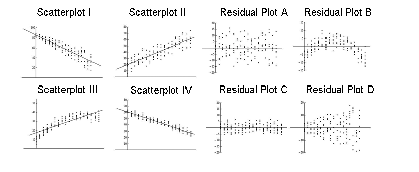
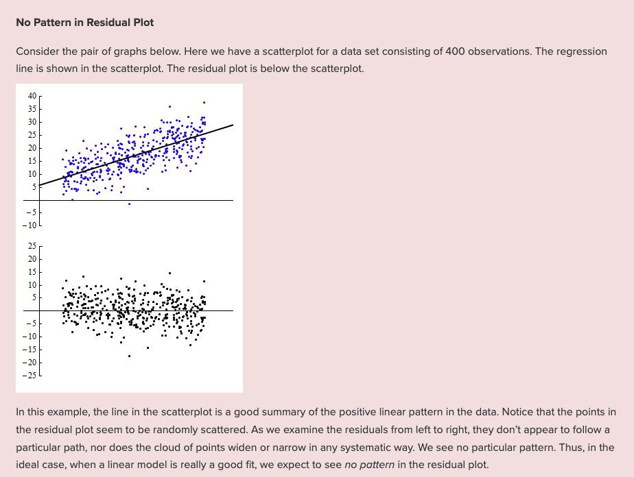
What are we looking for in a residual plot?

Unexpected patterns

Example 1

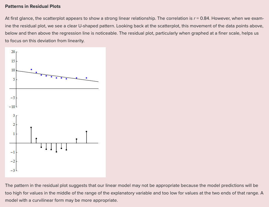
Example 2

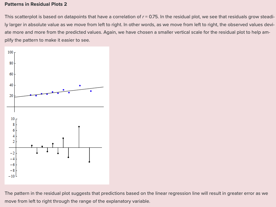
Example 3

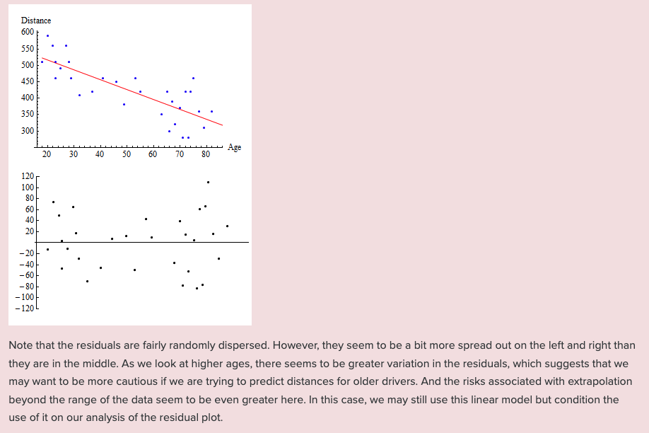
Example 4

Which fit?