Chapter 1 Introduction to Mapping and Spatial Analysis
1.1 GIS and R for Geospatial Data Analysis
This is a compilation of notes and tutorials to accompany GIS and Spatial Analysis curricular activities at Bard College.
GIS for Environmental Justice ES 321 (Fall)
Introduction to Mapping and Spatial Analsis in R (Spring)
GIS and R workshops, tutorials, modules, and sidecar courses
Development of this book is ongoing.
1.2 An Expansive View of Spatial Analysis
Geospatial Data Analysis
Geospatial data is used to represent the position of something in relation to the things around it. Geospatial data analysis is the process of analyzing, revealing, interpreting and visualizing information such as location, distance, and spatial interaction to generate questions about and better understand our changing built and natural environments.
Our analysis seeks to characterize the spatial distribution, patterns of things represented by geographic data. While we will explore statistical spatial analysis, we also cover the ways in which geographic data manipulation and mapping can provide insights in descriptive and exploratory analysis. In spatial analysis, when the location changes, the information content of the data changes: location, direction, distance, relationships to/between change.
We can think of spatial data analysis in terms of three broad categories.
Mapping and geovisualization: Showing (interesting) patterns
Exploratory spatial data analysis: Discovering patterns
Spatial modeling: Explaining patterns, optimization, simulation, prediction
1.3 What is a GIS?
Geographic Information System (GIS) provides data structures and capabilities for storing, analyzing, managing, and publishing map data.
A set of computer tools that allows people to work with data that are tied to a particular location on the earth
A database that is designed to work with geospatial data
A Geographic Information System is computing environment used to create, manage, visualize and analyze data and its spatial counterpart.
1.3.1 GIS Functions
Data entry from a variety of sources, including digitizing, scanning, text files, and the most common spatial data formats; ways to export information to other programs should also be provided.
Data management tools, including tools for building data sets, editing spatial features and their attributes, and managing coordinate systems and projections.
Thematic mapping (displaying data in map form), including symbolizing map features in different ways and combining map layers for display.
Data analysis functions for exploring spatial relationships in and between map layers.
Map layout functions for creating digital or paper maps with titles, scale bars, north arrows, and other map elements
It’s important to note that most data sets you will encounter in your lifetime can all be assigned a spatial location whether on the earth’s surface or within some arbitrary coordinate system (such as a soccer field or a gridded petre dish). So in essence, any data set can be represented in a GIS: the question then becomes “does it need to be analyzed in a GIS environment?” The answer to this question depends on the purpose of the analysis. If, for example, we are interested in identifying the ten African countries with the highest conflict index scores for the 1966-78 period, a simple table listing those scores by country is all that is needed.
| Country | Conflicts | Country | Conflicts |
|---|---|---|---|
| EGYPT | 5246 | LIBERIA | 980 |
| SUDAN | 4751 | SENEGAL | 933 |
| UGANDA | 3134 | CHAD | 895 |
| ZAIRE | 3087 | TOGO | 848 |
| TANZANIA | 2881 | GABON | 824 |
| LIBYA | 2355 | MAURITANIA | 811 |
| KENYA | 2273 | ZIMBABWE | 795 |
| SOMALIA | 2122 | MOZAMBIQUE | 792 |
| ETHIOPIA | 1878 | IVORY COAST | 758 |
| SOUTH AFRICA | 1875 | MALAWI | 629 |
| MOROCCO | 1861 | CENTRAL AFRICAN REPUBLIC | 618 |
| ZAMBIA | 1554 | CAMEROON | 604 |
| ANGOLA | 1528 | BURUNDI | 604 |
| ALGERIA | 1421 | RWANDA | 487 |
| TUNISIA | 1363 | SIERRA LEONE | 423 |
| BOTSWANA | 1266 | LESOTHO | 363 |
| CONGO | 1142 | NIGER | 358 |
| NIGERIA | 1130 | BURKINA FASO | 347 |
| GHANA | 1090 | MALI | 299 |
| GUINEA | 1015 | THE GAMBIA | 241 |
| BENIN | 998 | SWAZILAND | 147 |
Data source: Anselin, L. and John O’Loughlin. 1992. Geography of international conflict and cooperation: spatial dependence and regional context in Africa. In The New Geopolitics, ed. M. Ward, pp. 39-75.
A simple sort on the Conflict column reveals that EGYPT, SUDAN, UGANDA, ZAIRE, TANZANIA, LIBYA, KENYA, SOMALIA, ETHIOPIA, SOUTH AFRICA are the top ten countries.
What if we are interested in knowing whether countries with a high conflict index score are geographically clustered, does the above table provide us with enough information to help answer this question? The answer, of course, is no. We need additional data pertaining to the geographic location and shape of each country. A map of the countries would be helpful.
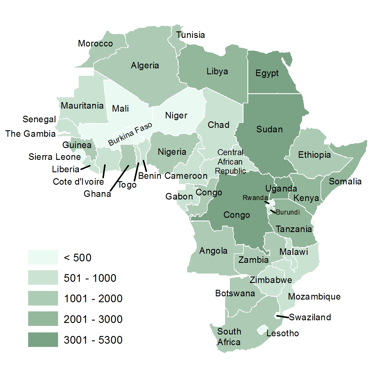
Figure 1.1: Choropleth representation of African conflict index scores. Countries for which a score was not available are not mapped.
Maps are ubiquitous: available online and in various print medium. But we seldom ask how the boundaries of the map features are encoded in a computing environment? After all, if we expect software to assist us in the analysis, the spatial elements of our data should be readily accessible in a digital form. Spending a few minutes thinking through this question will make you realize that simple tables or spreadsheets are not up to this task. A more complex data storage mechanism is required. This is the core of a GIS environment: a spatial database that facilitates the storage and retrieval of data that define the spatial boundaries, lines or points of the entities we are studying. This may seem trivial, but without a spatial database, most spatial data exploration and analysis would not be possible!
1.3.2 GIS software
Many GIS software applications are available–both commercial and open source. Two popular applications are ArcGIS and QGIS.
1.3.2.1 ArcGIS
A popular commercial GIS software is ArcGIS developed by ESRI (ESRI, pronounced ez-ree),was once a small land-use consulting firm which did not start developing GIS software until the mid 1970s. The ArcGIS desktop environment encompasses a suite of applications which include ArcGIS Pro, ArcCatalog, and ArcScene. ArcGIS comes in three different license levels (basic, standard and advanced) and can be purchased with additional add-on packages. As such, a single license can range from a few thousand dollars to well over ten thousand dollars. In addition to software licensing costs, ArcGIS is only available for Windows operating systems; so if your workplace is a Mac only environment, the purchase of a Windows PC or Parallels would add to the expense.
1.3.3 QGIS
A very capable open source (free) GIS software is QGIS. It encompasses most of the functionality included in ArcGIS. If you are looking for a GIS application for your Mac or Linux environment, QGIS is a wonderful choice given its multi-platform support. Built into the current versions of QGIS are functions from another open source software: GRASS. GRASS has been around since the 1980’s and has many advanced GIS data manipulation functions however, its use is not as intuitive as that of QGIS or ArcGIS (hence the preferred QGIS alternative).
1.4 What is Spatial Analysis?
A distinction is often made between GIS and spatial analysis. In the context of mainstream GIS software, the term analysis refers to data manipulation, data querying, and data organization/storage. In the context of spatial analysis, the analysis often focuses on the statistical analysis of patterns and underlying processes or more generally, spatial analysis addresses the question “what could have been the genesis of the observed spatial pattern?” It’s an exploratory process whereby we attempt to quantify the observed pattern then explore the processes that may have generated the pattern.
For example, you record the location of each tree in a well defined study area. You then map the location of each tree (a GIS or mapping task). At this point, you might be inclined to make inferences about the observed pattern. Are the trees clustered or dispersed? Is the tree density constant across the study area? Could soil type or slope have led to the observed pattern? Those are questions that are addressed in spatial analysis using quantitative and statistical techniques.
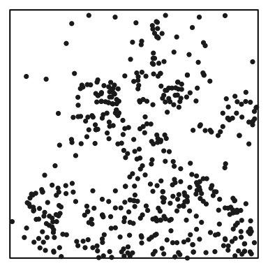
Figure 1.2: Distribution of Maple trees in a 1,000 x 1,000 ft study area.
With spatial analysis, we are often interested in finding out how the information contained in one spatial data set relates to that contained in another.
The kinds of questions we may be interested in include:
How does X interact with Y?
How many X are there in different locations of Y?
How does the incidence of X relate to the rate of Y?
How many of X are found within a certain distance of Y?
How does process X vary with Y spatially?
X and Y may be diseases, pollution events, attributed census areas (e.g, housing characteristics), environmental factors, deprivation indices or any other geographical process or phenomenon that you are interested in understanding.
Answering such questions using a spatial analysis frequently requires some initial data pre-processing and manipulation.
This might be to ensure that different data have the same spatial extent, describe processes in a consistent way (e.g. to compare land cover types from different classifications), are summarized over the same spatial framework (e.g. census reporting areas), are of the same format (raster, vector, etc.) and are projected in the same way.
This also often involves deepening our understand and presentation of spatial relationships through spatial data manipulation:
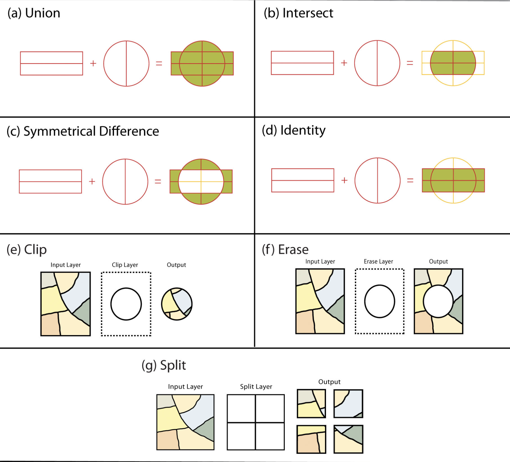
Figure 1.3: Examples of spatial data operations.
1.4.0.1 Core concepts for spatial analysis and mapping
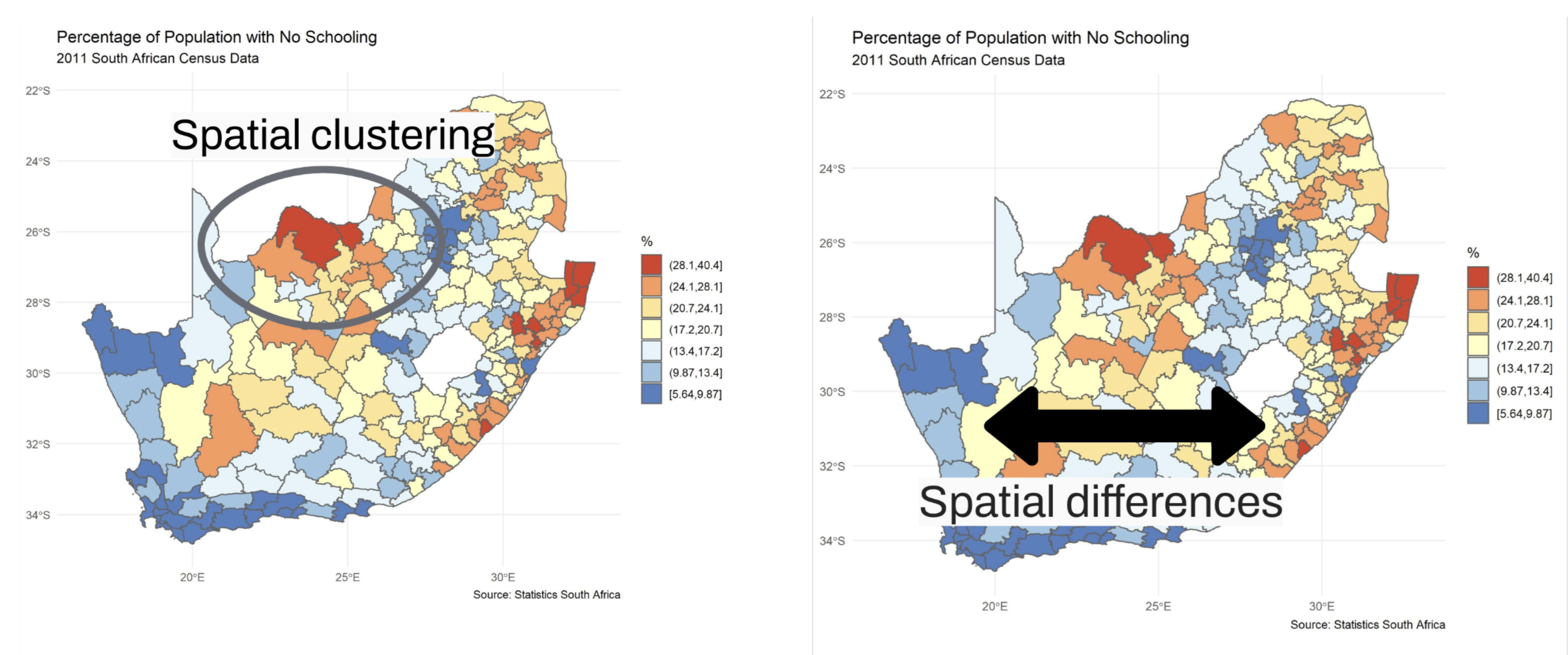
Figure 1.4: Examples of spatial variation.
Spatial heterogeneity (variation or difference). This is the idea that the values typical in one part of the map are not typical in another. To put it simply, some parts of the map are shaded in blue whereas others are in red and those parts seem neither randomly nor regularly distributed because of…
Spatial clustering. This is the idea that values found in one part of the map tend to be surrounded by similar values in neighboring parts of the map. In other words, there are patches of blue and patches of red colored areas on the map – blue tends be near blue and red tends to be near red.
- Another name for this is positive spatial autocorrelation: values tend to be more similar to nearby other values than they are to distant ones.
Spatial discontinuities (negative spatial autocorrelation) because sometimes neighboring places can have very different characteristics – there there can be sharp changes across borders (red next to blue).
Spatial dependencies
These characteristics of spatial variation indicate spatial dependence, whereby the measured attributes of one place are not independent of other places. Attributes in one location are influenced by other locations, near and far. We use theory and applied analysis methods to better understand the underlying spatial processes. Geospatial data analysis
This dependence has statistical consequences if assumptions of independence are violated.
Of more substantive geographic interest is how they have arisen – which processes are they caused by or associated with? Why are places not all the same? Why is there a geographical pattern?
Complicating the answers to these questions is that what we see in the map is not just a function of underlying social or other processes but also the ways the data are collected and the map constructed.
What you will learn in this course is that popular GIS software like ArcGISPro and ArcGIS Online are great tools to create and manipulate spatial data, but if one wishes to go beyond data manipulation and description to quantitatively analyze patterns and processes that may have led to these patterns, other quantitative tools are needed for a reproducible analysis with the latest spatial analysis methods. One such tool we will use in this class is R: an open source (freeware) data analysis environment. Another common tool that we might explore is GeoDA, an analysis environment built using R programming.
R has one, if not the richest set of spatial data analysis and statistics tools available today. Learning the R programming environment will prove to be quite beneficial given that many of the operations learnt are transferable across many other (non-spatial) quantitative analysis projects.
R can be installed on both Windows and Mac operating systems. Another related piece of software that you might find useful is RStudio which offers a nice interface to R.
1.5 What’s in an Acronym?
GIS use is growing in public sector and private sector work, research across disciplines in the arts, humanities, and sciences. Most think of GIS as solely a map making environment. While visualizing data is an important feature of a GIS, it is important to not lose sight of what data is being visualized and for what purpose.
The different purposes of mapping spatial data have strong parallels to that of graphing (or plotting) non-spatial data. John Tukey (Tukey 1972) offers three broad classes of the latter:
- Graphs from which numbers are to be observed- substitutes for tables.
- Graphs intended to show the reader what has already been learned (by some other technique)–these we shall sometimes impolitely call propaganda graphs.
- Graphs intended to let us see what may be happening over and above what we have already described- these are the analytical graphs that are our main topic.
A GIS world analogy:
- Reference maps (USGS maps, hiking maps, transportation maps). Such maps are used to navigate landscapes or identify locations and points-of-interest.
- Presentation maps presented in the press such as the NY Times and the Wall Street Journal, but also maps presented in journals. Such maps are designed to convey a very specific narrative of the author’s choosing. (Here we’ll avoid Tukey’s harsh description of such visual displays, but the idea that maps can be used as propaganda is not far fetched).
- Statistical maps whose purpose it is to manipulate the raw data in such a way to tease out patterns otherwise not discernible in its original form. This usually requires multiple data manipulation operations and visualization and can sometimes benefit from being explored outside of a spatial context.
This course will focus on the last two spatial data visualization applications.
1.5.1 The Importance of Context, History, Power
While you are learning to incorporate GIS into your research or professional work avoid placing the technology before purpose and theory. GIS and R software make manipulating geospatial data accessible, and can easily be seen and used as mere tools devoid of the context in which they are used. At times we will focus on learning the mechanics of mapping and spatial analysis. However, awareness and understanding of the context and purpose for which we rely on these software is equally if not more important that mastering the mechanics.
Website created and maintained by Jordan Ayala