Chapter 2 Feature Representation
2.1 Vector vs. Raster Data Models
To work in a GIS environment, real world observations (objects or events that can be recorded in 2D or 3D space) need to be reduced to spatial representations. These spatial representations can be presented in a GIS as a vector data model or a raster data model.
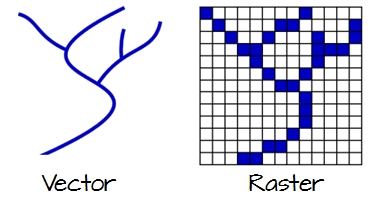
Figure 2.1: Vector and raster representations of a river feature.
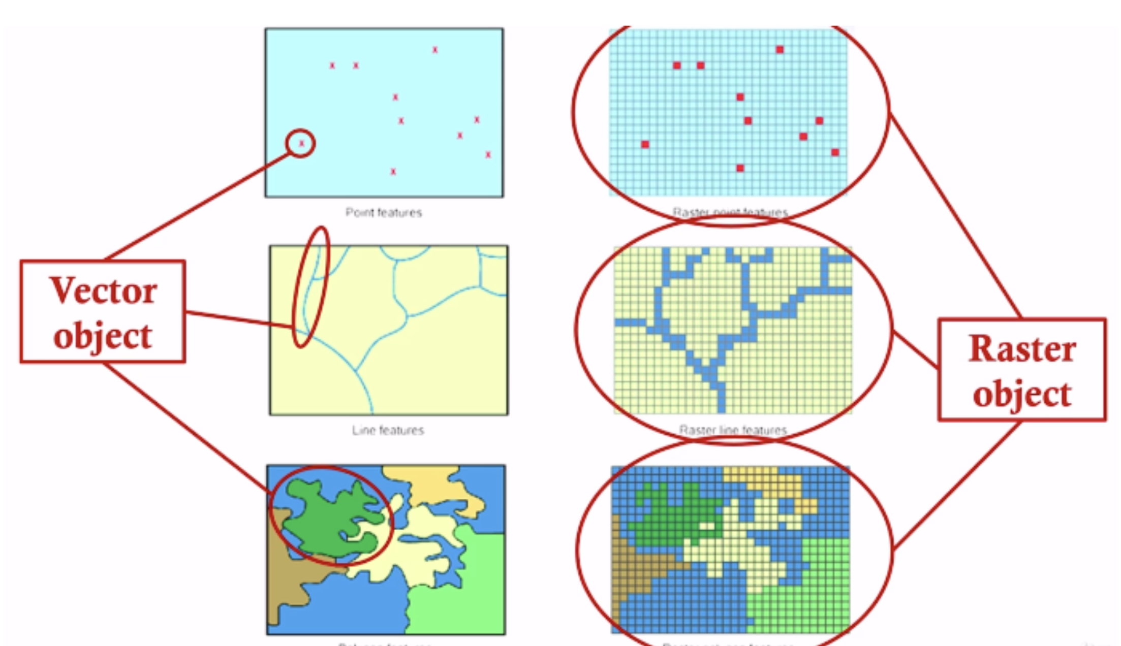
Figure 2.2: Vector and raster data model example.
2.1.1 Vector
Vector features can be decomposed into three different geometric primitives: points, lines/polylines and polygons.
2.1.1.1 Points

Figure 2.3: Three point objects defined by their X and Y coordinate values.
A point is composed of one coordinate pair representing a specific location in a coordinate system. Points are the most basic geometric primitives having no length or area. By definition a point can’t be “seen” since it has no area; but this is not practical if such primitives are to be mapped. So points on a map are represented using symbols that have both area and shape (e.g. circle, square, plus signs).
We seem capable of interpreting such symbols as points, but there may be instances when such interpretation may be ambiguous (e.g. is a round symbol delineating the area of a round feature on the ground such as a large oil storage tank or is it representing the point location of that tank?).
2.1.1.2 Polylines
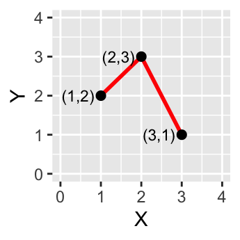
Figure 2.4: A simple polyline object defined by connected vertices.
A polyline is composed of a sequence of two or more coordinate pairs called vertices. A vertex is defined by coordinate pairs, just like a point, but what differentiates a vertex from a point is its explicitly defined relationship with neighboring vertices. A vertex is connected to at least one other vertex.
Like a point, a true line can’t be seen since it has no area. And like a point, a line is symbolized using shapes that have a color, width and style (e.g. solid, dashed, dotted, etc…). Roads and rivers are commonly stored as polylines in a GIS.
2.1.1.3 Polygons
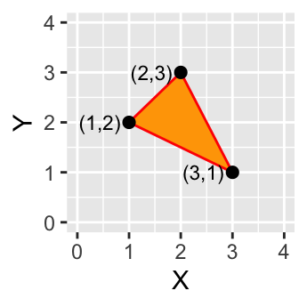
Figure 2.5: A simple polygon object defined by an area enclosed by connected vertices.
A polygon is composed of three or more line segments whose starting and ending coordinate pairs are the same. Sometimes you will see the words lattice or area used in lieu of ‘polygon’. Polygons represent both length (i.e. the perimeter of the area) and area. They also embody the idea of an inside and an outside; in fact, the area that a polygon encloses is explicitly defined in a GIS environment. If it isn’t, then you are working with a polyline feature. If this does not seem intuitive, think of three connected lines defining a triangle: they can represent three connected road segments (thus polyline features), or they can represent the grassy strip enclosed by the connected roads (in which case an ‘inside’ is implied thus defining a polygon).
2.1.2 Raster
Figure 2.6: A simple raster object defined by a 10x10 array of cells or pixels.
A raster data model uses an array of cells, or pixels, to represent real-world objects. Raster data sets are commonly used for representing and managing imagery, surface temperatures, digital elevation models, and numerous other entities.
A raster can be thought of as a special case of an area object where the area is divided into a regular grid of cells. But a regularly spaced array of marked points may be a better analogy since rasters are stored as an array of values where each cell is defined by a single coordinate pair inside of most GIS environments.
Implicit in a raster data model is a value associated with each cell or pixel. This is in contrast to a vector model that may or may not have a value associated with the geometric primitive.
Also note that a raster data structure is square or rectangular. So, if the features in a raster do not cover the full square or rectangular extent, their pixel values will be set to no data values (e.g. NULL or NoData).
2.2 Object vs. Field
The traditional vector/raster perspective of our world is one that has been driven by software and data storage environments. But this perspective is not particularly helpful if one is interested in analyzing the pattern. In fact, it can mask some important properties of the entity being studied. An object vs. field view of the world proves to be more insightful even though it may seem more abstract.
2.2.1 Object view
An object view of the world treats entities as discrete objects; they need not occur at every location within a study area. Point locations of cities would be an example of an object. So would be polygonal representations of urban areas which may be non-contiguous.
2.2.2 Field view
A field view of the world treats entities as a scalar field. This is a mathematical concept in which a scalar is a quantity having a magnitude. It is measurable at every location within the study region. Two popular examples of a scalar field are surface elevation and surface temperature. Each represents a property that can be measured at any location.
Another example of a scalar field is the presence and absence of a building. This is a binary scalar where a value of 0 is assigned to a location devoid of buildings and a value of 1 is assigned to locations having one or more buildings. A field representation of buildings may not seem intuitive, in fact, given the definition of an object view of the world in the last section, it would seem only fitting to view buildings as objects. In fact, buildings can be viewed as both field or objects. The context of the analysis is ultimately what will dictate which view to adopt. If we’re interested in studying the distribution of buildings over a study area, then an object view of the features makes sense. If, on the other hand, we are interested in identifying all locations where buildings don’t exist, then a binary field view of these entities would make sense.
2.3 Scale
Scale has two separate meanings in geography:
Map Scale or Cartographic Scale: the measurement on a map (ratio of space on map to space on the globe); and
Geographic Scale: the hierarchy of spaces or places
2.3.1 Map Scale
How one chooses to represent a real-world entity will be in large part dictated by the scale of the analysis. In a GIS, scale has a specific meaning: it’s the ratio of distance on the map to that in the real world. So a large scale map implies a relatively large ratio and thus a small extent. This is counter to the common interpretation of large scale which focuses on the scope or extent of a study; so a large scale analysis would imply one that covers a large area.
A measure of the size at which features in a map are represented. The scale is expressed as a fraction, or ratio, of the size of features represented by the map to the size of the actual objects on the ground. A large-scale map is one in which the ratio is large (i.e., the denominator is small). Thus, a 1:24,000 scale map has a larger scale than a 1:100,000 scale map.
The following two maps represent the same entity: the Boston region. At a small scale (e.g. 1:10,000,000), Boston and other cities may be best represented as points. At a large scale (e.g. 1:34,000), Boston may be best represented as a polygon. Note that at this large scale, roads may also be represented as polygon features instead of polylines.
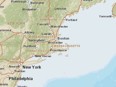
Figure 2.7: Map of the Boston area at a 1:10,000,000 scale. Note that in geography, this is considered small scale whereas in layperson terms, this extent is often referred to as a large scale (i.e. covering a large area).
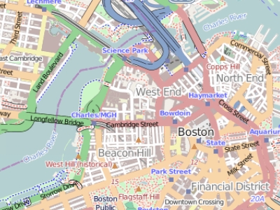
Figure 2.8: Map of the Boston area at a 1:34,000 scale. Note that in geography, this is considered large scale whereas in layperson terms, this extent is often referred to as a small scale (i.e. covering a small area).
2.3.2 Geographic scale
Geographic conceptual hierarchy of spaces, from small to large that reflects actual levels of organization in the real world.
Example from small to large: Neighborhood → Urban Area → Metropolitan Area → Region → Nation → World
Geographic scales used in research:
Human Settlements – community, home, body
Nation States - subdivided into de jure (“concerning law”) regions or functional regions
World Regions – major clusters of humankind with broadly similar cultural attributes
World Economy – subdivided into core, semipheriphery, and periphery
Example: Unemployment and other socio-economic characteristics, Murders in the U.S.
2.4 Attribute Tables
Non-spatial information associated with a spatial feature is referred to as an attribute. A feature on a GIS map is linked to its record in the attribute table by a unique numerical identifier (ID). Every feature in a layer has an identifier. It is important to understand the one-to-one or many-to-one relationship between feature, and attribute record. Because features on the map are linked to their records in the table, many GIS software will allow you to click on a map feature and see its related attributes in the table.
Raster data can also have attributes only if pixels are represented using a small set of unique integer values. Raster data sets that contain attribute tables typically have cell values that represent or define a class, group, category, or membership. NOTE: not all GIS raster data formats can store attribute information; in fact many raster data sets you will work with in this course will not have attribute tables.
2.4.1 Data measurement types
Attribute data can be broken down into four measurement types:
Nominal data which have no implied order, size or quantitative information (e.g. paved and unpaved roads, place names or labels)
Ordinal data have an implied order (e.g. ranked scores).
Interval data name or otherwise identify objects. Interval data are numeric and have a linear scale, however they do not have a true zero and can therefore not be used to measure relative magnitudes. For example, one cannot say that 60°F is twice as warm as 30°F since when presented in degrees °C the temperature values are 15.5°C and -1.1°C respectively (and 15.5 is clearly not twice as big as -1.1).
Ratio scale data are interval data with a true zero such as monetary value (e.g. $1, $20, $100).
We characterize measurements or attributes as belonging to one of a set of data measurement types:
Categorical data: nominal or ordinal
Discrete or continuous numerical (quantitative) data: interval or ratio
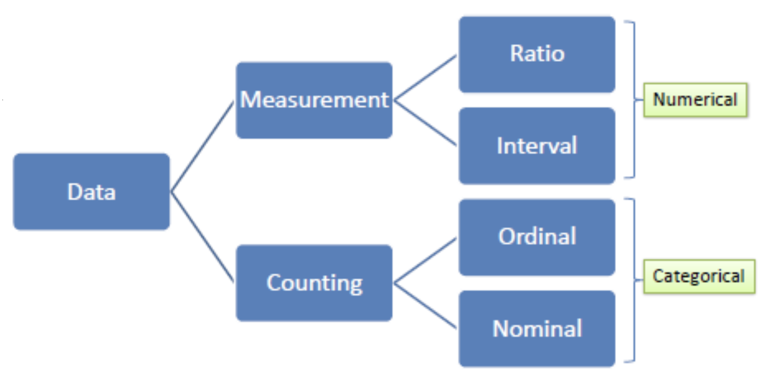
(#fig:measurement types)Graphic of data measurement types.
Categorical data separate features into distinct groups or classes: nominal or ordinal. In GIS: symbolized by a point (class of point objects), line (type of road, highway, etc.) or polygon (type of land color, predominance measure).
Ordinal data
For example, urban settlements might be classified as villages, towns, or cities. Students are assigned grades of A, B, C, D, or F. U.S. New Deal era Home Owners Loan Corporation redlining categories are another example, whereby areas within cities were ranked in terms of “security” for mortgage insurance.
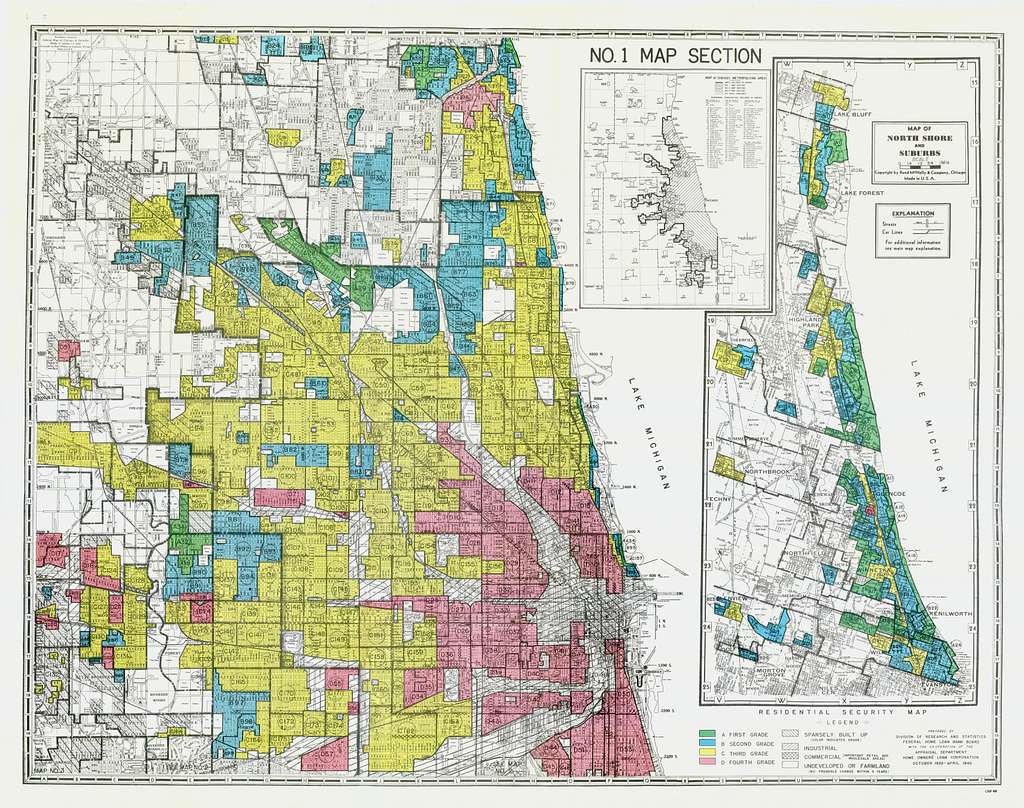
Figure 2.9: Redlining map of Chicago, as created by the Home Owners’ Loan Corporation..
In mathematics and statistics, a quantitative variable may be continuous or discrete if they are typically obtained by measuring (continuous) or counting (discrete).
Discrete data are objects in the real world with specific locations or boundaries, such as houses, cities, roads, neighborhoods or counties. (Vector: point, lines and polygon features with a connected table of attribute data)
Continuous data represent quantities that may be measured anywhere on the earth, such as temperature or elevation. Continuous data are often represented using the raster data model, cells of pixels.
Some rasters store physical quantities like elevation, temperature, or precipitation.
Others may store color and brightness values that make up aerial photographs, satellite images, or a scanned paper map.
Quantitative or numerical data represent phenomena that fall along a regularly spaced measurement scale.
Interval data have a regular scale but are not related to a meaningful zero point. Example: Temperature (temperature of 0 is not equal to no temperature)
Ratio data have a meaningful zero point that indicates the absence of the thing being measured.
Quantitative numeric data take on values along a continuous scale of possibilities; Every state, for example, has its own population value. In order to symbolize numeric data, the values must be partitioned into groups with specific ranges. Mapping numeric data, raster or vector, requires classifying a range of values into a small number of groups, each of which can be represented by a different color or symbol size. This process is called classification.
2.4.2 Data type
Another way to categorize an attribute is by its data type. ArcGIS supports several data types such as integer, float, double and text. Knowing your data type and measurement level should dictate how they are stored in a GIS environment. The following table lists popular data types available in most GIS applications.
| Type | Stored values | Note |
|---|---|---|
| Short integer | -32,768 to 32,768 | Whole numbers |
| Long integer | -2,147,483,648 to 2,147,483,648 | Whole numbers |
| Float | -3.4 * E-38 to 1.2 E38 | Real numbers |
| Double | -2.2 * E-308 to 1.8 * E308 | Real numbers |
| Text | Up to 64,000 characters | Letters and words |
While whole numbers can be stored as a float or double (i.e. we can store the number 2 as 2.0) doing so comes at a cost: an increase in storage space. This may not be a big deal if the data set is small, but if it consists of tens of thousands of records the increase in file size and processing time may become an issue.
While storing an integer value as a float may not have dire consequences, the same cannot be said of storing a float as an integer. For example, if your values consist of 0.2, 0.01, 0.34, 0.1 and 0.876, their integer counterpart would be 0, 0, 0, and 1 (i.e. values rounded to the nearest whole number). This can have a significant impact on a map as shown in the following example.
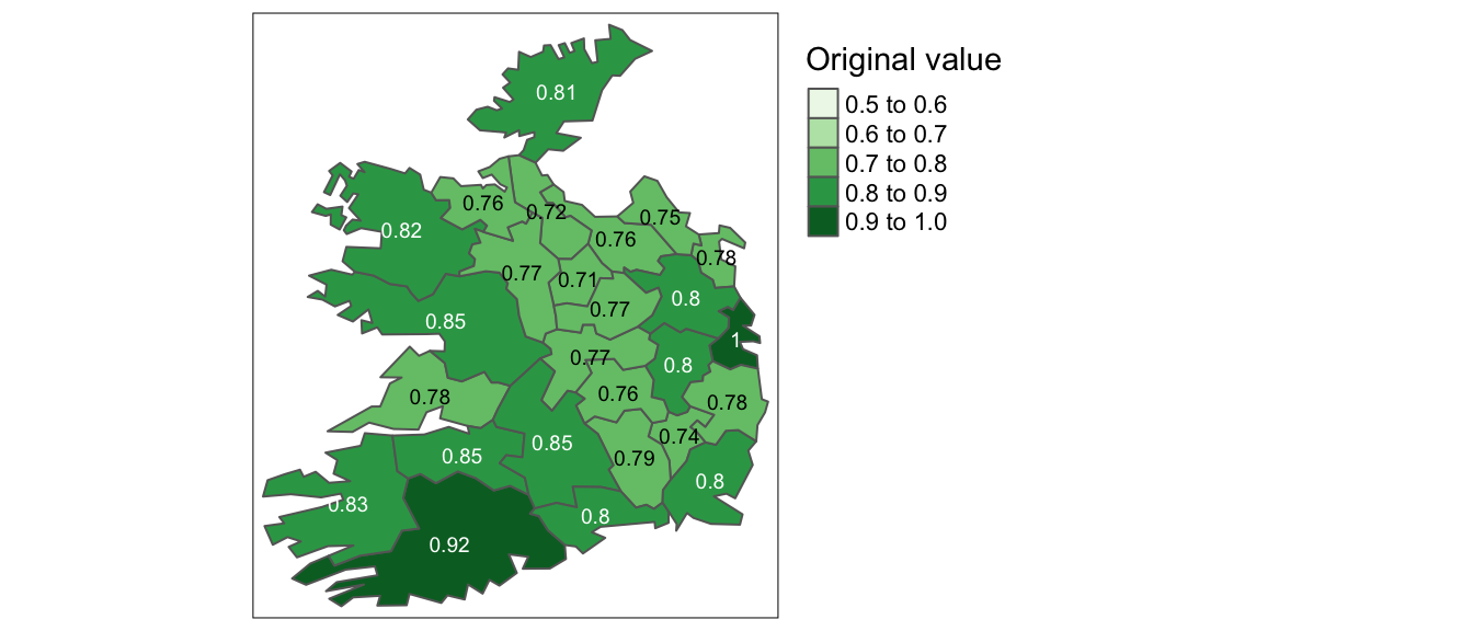
Figure 2.10: Map of data represented as decimal (float) values.
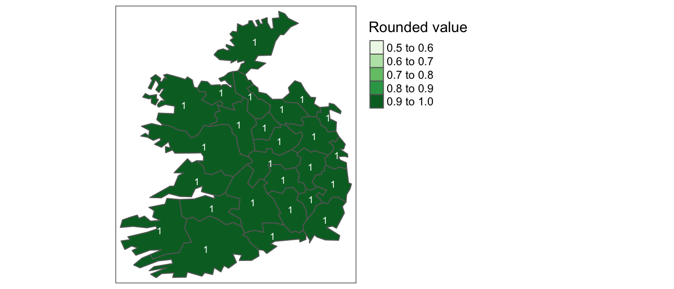
Figure 2.11: Map of same data represented as integers instead of float.
2.5 Resolution
Resolution refers to the sampling interval at which data are acquired. Resolution may be spatial (what is represented by one pixel or one spatial unit like census tracts or counties), thematic, or temporal (Decennial Census data vs. American Community Survey estimates, ACS).
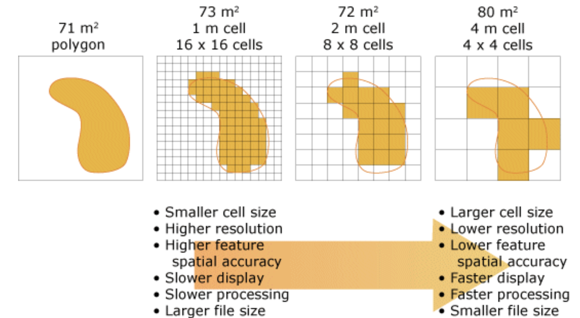
Figure 2.12: Map resolution example
High resolution entails a higher frequency of measurement or counting and smaller areal units. while low resolution entails a lower frequency of measurement or counting. In the raster data model, a higher resolution spatial representation of data entails pixels that represent a smaller area on the earth. 1 meter resolution is higher resolution than 1 mile. In the vector data model, census tracts represent a higher spatial resolution than counties.
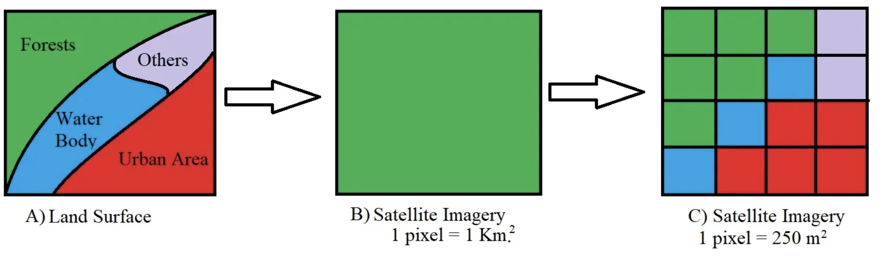
Figure 2.13: Map resolution example: from vector to raster
Website created and maintained by Jordan Ayala