Chapter 3 GIS Data Management
3.1 GIS File Data Formats
In the GIS world, you will encounter many different GIS file formats. Some file formats are unique to specific GIS applications, others are universal. For this course, we will focus on a subset of spatial data file formats: shapefiles for vector data, Imagine and GeoTiff files for rasters and file geodatabases and geopackages for both vector and raster data.
3.1.1 Vector Data File Formats
3.1.1.1 Shapefile
A shapefile is a file-based data format native to ArcView 3.x software (a much older version of ArcGIS for Desktop). Conceptually, a shapefile is a feature class–it stores a collection of features that have the same geometry type (point, line, or polygon), the same attributes, and a common spatial extent.
Despite what its name may imply, a “single” shapefile is actually composed of at least three files, and as many as eight. Each file that makes up a “shapefile” has a common filename but different extension type.
The list of files that define a “shapefile” are shown in the following table. Note that each file has a specific role in defining a shapefile.
| File extension | Content |
|---|---|
| .dbf | Attribute information |
| .shp | Feature geometry |
| .shx | Feature geometry index |
| .aih | Attribute index |
| .ain | Attribute index |
| .prj | Coordinate system information |
| .sbn | Spatial index file |
| .sbx | Spatial index file |
3.1.1.2 File Geodatabase
A file geodatabase is a relational database storage format. It’s a far more complex data structure than the shapefile and consists of a .gdb folder housing dozens of files. Its complexity renders it more versatile allowing it to store multiple feature classes and enabling topological definitions (i.e. allowing the user to define rules that govern the way different feature classes relate to one another). An example of the contents of a geodatabase is shown in the following figure.
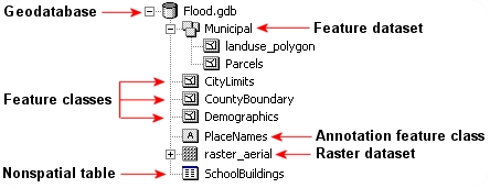
Figure 3.1: Sample content of an ArcGIS file geodatabase. (src: esri)
3.1.1.3 GeoPackage
A GeoPackage is an open, SQLite-based format that can store vector features, attribute tables, and raster tiles in one .gpkg file. A single file makes it convenient to exchange data across GIS applications. Support for particular editing and metadata operations varies by application. In ArcGIS Pro, the Create SQLite Database geoprocessing tool can create a GeoPackage; a script is not required. See ArcGIS Pro’s GeoPackage guidance.
In an ArcGIS Pro workflow, keep working feature classes and tables in the project geodatabase. Keep downloaded originals separately. Use an exchange format deliberately, checking field names, data types, missing values, and coordinate information after export.
3.1.2 Raster Data File Formats
Rasters are in part defined by their pixel depth. Pixel depth defines the range of distinct values the raster can store. For example, a 1-bit raster can only store 2 distinct values: 0 and 1.
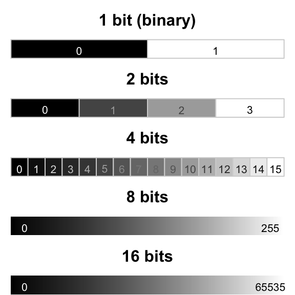
Figure 3.2: Examples of different pixel depths.
There is a wide range of raster file formats used in the GIS world. Some of the most popular ones are listed below.
3.1.2.1 Imagine
The Imagine file format was originally created by an image processing software company called ERDAS. This file format consists of a single .img file. This is a simpler file format than the vector shapefile. It is sometimes accompanied by an .xml file which usually stores metadata information about the raster layer.
3.1.2.2 GeoTiff
A popular public domain raster data format is the GeoTIFF format. If maximum portability and platform independence is important, this file format may be a good choice.
3.1.2.3 File Geodatabase
A raster file can also be stored in a file geodatabase alongside vector files. Geodatabases have the benefit of defining image mosaic structures thus allowing the user to create “stitched” images from multiple image files stored in the geodatabase. Also, processing very large raster files can be computationally more efficient when stored in a file geodatabase as opposed to an Imagine or GeoTiff file format.
3.2 Managing GIS Files in ArcGIS
Unless you are intimately familiar with the file structure of a GIS file, it is best to copy/move/delete GIS files from within the software environment.
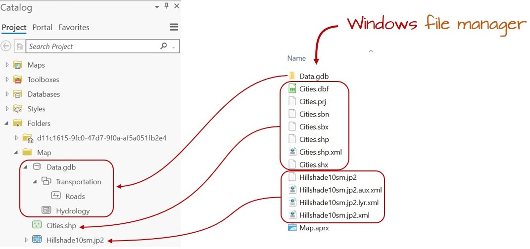
Figure 3.3: Windows File Explorer view vs. ArcGIS Catalog view. Note, for example, how the many files that make up the Cities shapefile (as viewed in a Windows file manager environment) appears as a single entry in the Catalog view. This makes it easier to rename the shapefile since it needs to be done only for a single entry in the GIS software (as opposed to renaming the Cities files seven times in the Windows file manager environment).
3.3 Managing a Map Project in ArcGIS
Unlike many other software environments such as word processors and spreadsheets, a GIS map project is not self-contained in a single file. A GIS map consists of many files: ArcGIS’ .aprx project file and the various vector and/or raster files used in the map project. The .aprx file stores the project configuration, including maps, layouts, layer properties, and connections to data. It does not embed every dataset used by those maps. A layer can also reference an online service that will still require network access and, sometimes, permission when the project is reopened. See ArcGIS Pro projects.
Because of the complex data structure associated with GIS maps, it’s usually best to store the .aprx and all associated GIS files under a single project directory. Then, when you are ready to share your map project with someone else, just pass along that project folder as is or compressed in a zip or tar file.
Because .aprx map files read data from GIS files, it must know where to find these files on your computer or across the network. There are two ways in which a map document can store the location to the GIS files: as a relative pathname or a full pathname. In older esri GIS applications, like ArcMap, the user had the choice to save a project using relative or full pathnames.
Note that ArcMap is a legacy GIS software replaced by ArcGIS Pro.
3.4 Documenting your work with data
Before you download a dataset, write the question it might help answer. Then identify what one record represents. A census tract, a housing unit, and a parcel are different observation units. A tract table cannot identify the status of an individual house.
As a worked example, consider a Hudson Valley housing analysis: the analytical geography is census tracts in Dutchess and Ulster counties. The table contains 2020–2024 ACS five-year estimates. The boundary file is the 2024 cartographic tract boundary release. Record both dates: an estimate’s period and a boundary’s vintage describe different things. A five-year estimate is not a count taken on the last day of 2024.
Keep a short data profile with the following information:
| Record | Housing example or question to answer |
|---|---|
| Producer and source of the data | U.S. Census Bureau; exact table or download link and date accessed |
| Observation unit and coverage | One tract; Dutchess and Ulster counties, New York |
| Period and boundary vintage | ACS 2020–2024; 2024 cartographic boundaries |
| Variables and universe | B25002 covers housing units; B25004 covers vacant housing units |
| Identifier | An 11-character tract GEOID stored as text |
| Geometry and CRS | Polygon boundaries; inspect the source CRS and units |
| Processing | Which records were selected, which fields were calculated, and where the output was saved |
| Limitations | Sampling uncertainty; generalized boundaries; meanings the source does not establish |
The 2024 Census cartographic boundary files are simplified for mapping. They are not parcel surveys. When the analysis uses tract-level counts, selecting whole tracts preserves the correspondence between geometry and attributes. Cutting a tract polygon into pieces does not automatically apportion its housing counts to those pieces.
Save original downloads separately from working data and exports. If a teaching extract was supplied, credit the original producer and describe the supplied extract. Record what you acquired or changed yourself. This makes the workflow traceable without claiming to have performed steps someone else completed.
Check your understanding: Could someone identify the source, period, observation unit, and geographic selection from your data profile without opening your map?
3.5 Joining tables and checking the relationship
A table join attaches attributes using a shared key. Census tract polygons and a tract-level housing table can use GEOID. In the 11-character tract GEOID, the state, county, and tract codes occupy fixed positions. Store the complete identifier as text: it labels a place and is not a quantity to add or average. Check that both tables use the same identifier format; some Census downloads provide a longer geography identifier that needs a documented conversion.
We expect one record per tract in each input, making this a one-to-one join. Test that expectation before using the result.
- Count the rows and distinct keys in each input. Investigate blank keys and duplicate GEOIDs.
- Check the data types, leading zeros, whitespace, and geography/period compatibility. Do not alter identifiers simply to force a match.
- Join the housing table to the selected tracts. Record whether unmatched target records are retained or excluded.
- Count matched and unmatched keys in both directions. Explain any table records outside the selected geography.
- Compare input and output counts, then verify three joined records against the original table.
Imagine two inputs with 132 rows each. One table could still have only 131 unique GEOIDs because a duplicate replaced a missing tract. Equal row counts would not reveal that error. Depending on the tool and join settings, duplicate matches may expand the output or select only one matching record. Neither result establishes the intended relationship. Use Validate Join and inspect its findings alongside your own checks.
Do not delete a duplicate until you understand it. Multiple records may describe different years, categories, or events. In that case, decide whether you need a filter, aggregation, or a different relationship. A spatial join, which uses location rather than a matching text key, answers a different question.
Check your understanding: A join finishes without an error and the map has colors. What evidence would let you trust it? Your answer should include key uniqueness, unmatched records, and checks against original values.
3.6 Calculated fields and recoverable work
Before calculating a field in an attribute table, record what is it measuring, the units of measurement, where it came from (e.g., observation, remotely sensed data from a drone or satellite), formula used to calculate (when applicable), and units in a dictionary. Use a decimal-capable field for percentages. Confirm whether the operation will affect all records or only a current selection.
Zero and missing are different. A recorded zero vacant units is a numerical estimate. An unavailable estimate is missing. A percentage with a zero denominator is undefined, so store it as null/unavailable and explain why. Do not turn missing values or Census special codes into ordinary zeros; consult the source annotations before calculating.
For three tracts, reproduce each formula with a calculator and compare it with the saved field. Check plausible ranges, such as 0–100 for a percentage, but remember that passing a range check does not prove the denominator is correct. The housing measures and their reconciliation checks are in Housing vacancy: the denominator changes the question.
Finish by reopening the project from the folder intended for storage or sharing. Confirm that local datasets, maps, and layouts load, and document online dependencies. Keep a short method log: input, operation/settings, output, check, and interpretation. This log explains your work more usefully than an unlabeled sequence of screenshots.
Website created and maintained by Jordan Ayala.