Rows: 10,000
Columns: 55
$ emp_title <chr> "global config engineer ", "warehouse…
$ emp_length <dbl> 3, 10, 3, 1, 10, NA, 10, 10, 10, 3, 1…
$ state <fct> NJ, HI, WI, PA, CA, KY, MI, AZ, NV, I…
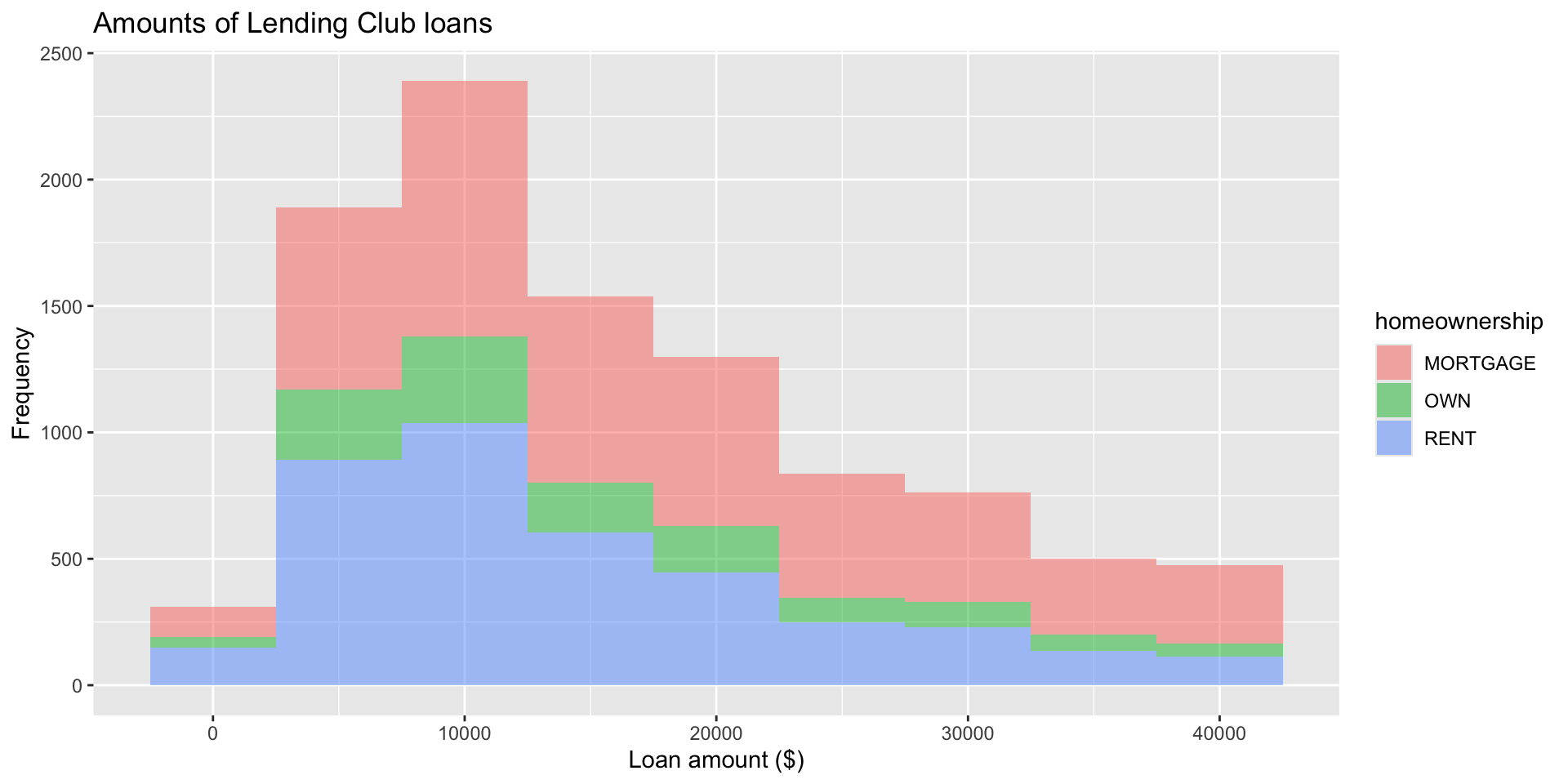
$ homeownership <fct> MORTGAGE, RENT, RENT, RENT, RENT, OWN…
$ annual_income <dbl> 90000, 40000, 40000, 30000, 35000, 34…
$ verified_income <fct> Verified, Not Verified, Source Verifi…
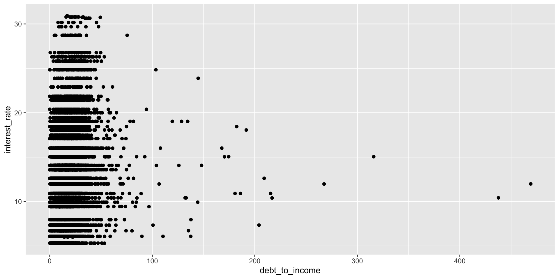
$ debt_to_income <dbl> 18.01, 5.04, 21.15, 10.16, 57.96, 6.4…
$ annual_income_joint <dbl> NA, NA, NA, NA, 57000, NA, 155000, NA…
$ verification_income_joint <fct> , , , , Verified, , Not Verified, , ,…
$ debt_to_income_joint <dbl> NA, NA, NA, NA, 37.66, NA, 13.12, NA,…
$ delinq_2y <int> 0, 0, 0, 0, 0, 1, 0, 1, 1, 0, 0, 0, 0…
$ months_since_last_delinq <int> 38, NA, 28, NA, NA, 3, NA, 19, 18, NA…
$ earliest_credit_line <dbl> 2001, 1996, 2006, 2007, 2008, 1990, 2…
$ inquiries_last_12m <int> 6, 1, 4, 0, 7, 6, 1, 1, 3, 0, 4, 4, 8…
$ total_credit_lines <int> 28, 30, 31, 4, 22, 32, 12, 30, 35, 9,…
$ open_credit_lines <int> 10, 14, 10, 4, 16, 12, 10, 15, 21, 6,…
$ total_credit_limit <int> 70795, 28800, 24193, 25400, 69839, 42…
$ total_credit_utilized <int> 38767, 4321, 16000, 4997, 52722, 3898…
$ num_collections_last_12m <int> 0, 0, 0, 0, 0, 0, 0, 0, 0, 0, 0, 0, 0…
$ num_historical_failed_to_pay <int> 0, 1, 0, 1, 0, 0, 0, 0, 0, 0, 1, 0, 0…
$ months_since_90d_late <int> 38, NA, 28, NA, NA, 60, NA, 71, 18, N…
$ current_accounts_delinq <int> 0, 0, 0, 0, 0, 0, 0, 0, 0, 0, 0, 0, 0…
$ total_collection_amount_ever <int> 1250, 0, 432, 0, 0, 0, 0, 0, 0, 0, 0,…
$ current_installment_accounts <int> 2, 0, 1, 1, 1, 0, 2, 2, 6, 1, 2, 1, 2…
$ accounts_opened_24m <int> 5, 11, 13, 1, 6, 2, 1, 4, 10, 5, 6, 7…
$ months_since_last_credit_inquiry <int> 5, 8, 7, 15, 4, 5, 9, 7, 4, 17, 3, 4,…
$ num_satisfactory_accounts <int> 10, 14, 10, 4, 16, 12, 10, 15, 21, 6,…
$ num_accounts_120d_past_due <int> 0, 0, 0, 0, 0, 0, 0, NA, 0, 0, 0, 0, …
$ num_accounts_30d_past_due <int> 0, 0, 0, 0, 0, 0, 0, 0, 0, 0, 0, 0, 0…
$ num_active_debit_accounts <int> 2, 3, 3, 2, 10, 1, 3, 5, 11, 3, 2, 2,…
$ total_debit_limit <int> 11100, 16500, 4300, 19400, 32700, 272…
$ num_total_cc_accounts <int> 14, 24, 14, 3, 20, 27, 8, 16, 19, 7, …
$ num_open_cc_accounts <int> 8, 14, 8, 3, 15, 12, 7, 12, 14, 5, 8,…
$ num_cc_carrying_balance <int> 6, 4, 6, 2, 13, 5, 6, 10, 14, 3, 5, 3…
$ num_mort_accounts <int> 1, 0, 0, 0, 0, 3, 2, 7, 2, 0, 2, 3, 3…
$ account_never_delinq_percent <dbl> 92.9, 100.0, 93.5, 100.0, 100.0, 78.1…
$ tax_liens <int> 0, 0, 0, 1, 0, 0, 0, 0, 0, 0, 0, 0, 0…
$ public_record_bankrupt <int> 0, 1, 0, 0, 0, 0, 0, 0, 0, 0, 1, 0, 0…
$ loan_purpose <fct> moving, debt_consolidation, other, de…
$ application_type <fct> individual, individual, individual, i…
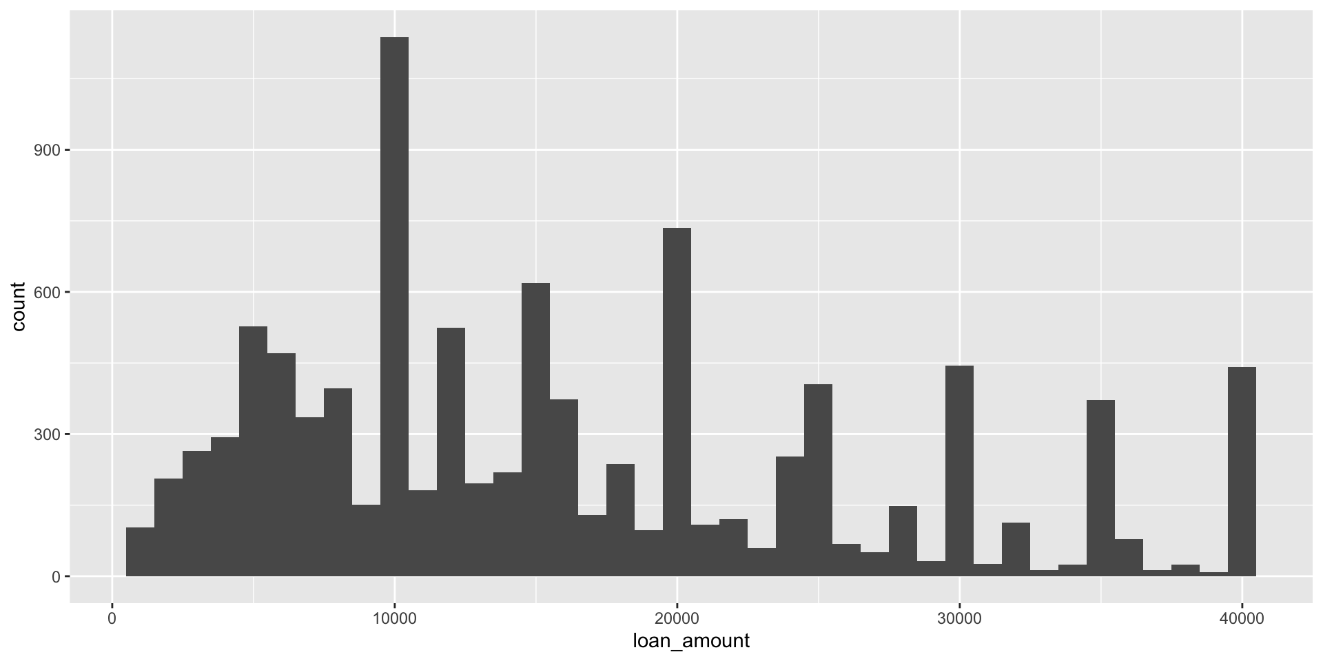
$ loan_amount <int> 28000, 5000, 2000, 21600, 23000, 5000…
$ term <dbl> 60, 36, 36, 36, 36, 36, 60, 60, 36, 3…
$ interest_rate <dbl> 14.07, 12.61, 17.09, 6.72, 14.07, 6.7…
$ installment <dbl> 652.53, 167.54, 71.40, 664.19, 786.87…
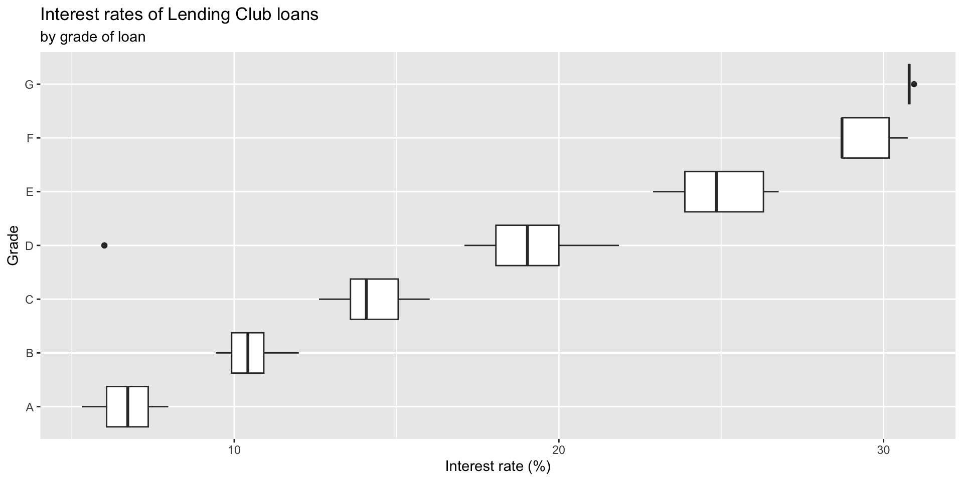
$ grade <ord> C, C, D, A, C, A, C, B, C, A, C, B, C…
$ sub_grade <fct> C3, C1, D1, A3, C3, A3, C2, B5, C2, A…
$ issue_month <fct> Mar-2018, Feb-2018, Feb-2018, Jan-201…
$ loan_status <fct> Current, Current, Current, Current, C…
$ initial_listing_status <fct> whole, whole, fractional, whole, whol…
$ disbursement_method <fct> Cash, Cash, Cash, Cash, Cash, Cash, C…
$ balance <dbl> 27015.86, 4651.37, 1824.63, 18853.26,…
$ paid_total <dbl> 1999.330, 499.120, 281.800, 3312.890,…
$ paid_principal <dbl> 984.14, 348.63, 175.37, 2746.74, 1569…
$ paid_interest <dbl> 1015.19, 150.49, 106.43, 566.15, 754.…
$ paid_late_fees <dbl> 0, 0, 0, 0, 0, 0, 0, 0, 0, 0, 0, 0, 0…Visualizing numerical data
Intro to Data Analytics
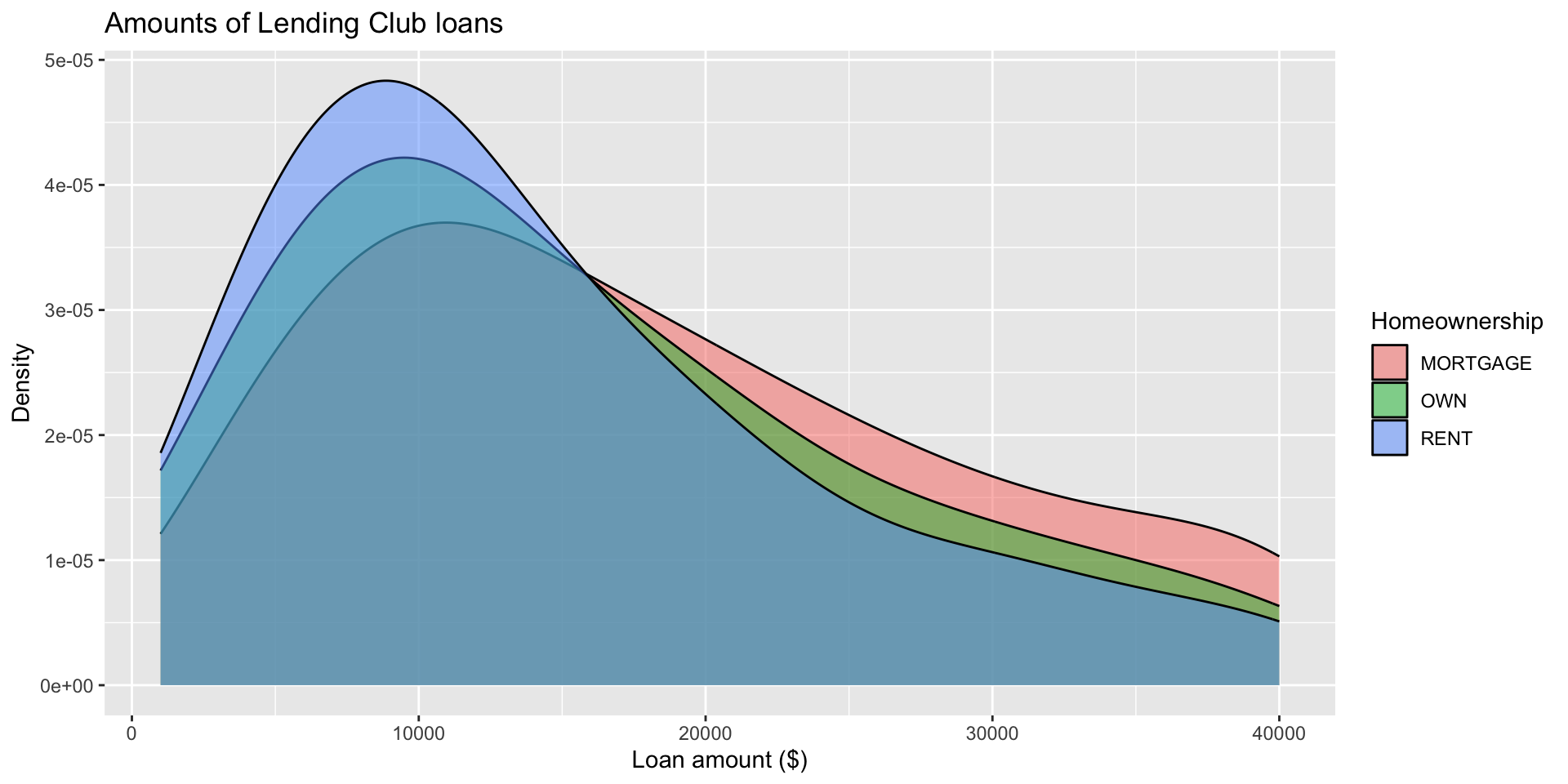
Data: Lending Club
Thousands of loans made through the Lending Club, a platform that allows individuals to lend to other individuals
Not all loans are created equal – ease of getting a loan depends on (apparent) ability to pay back the loan
Data includes loans made, these are not loan applications

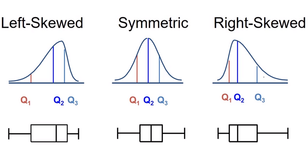
Describing shapes of numerical distributions
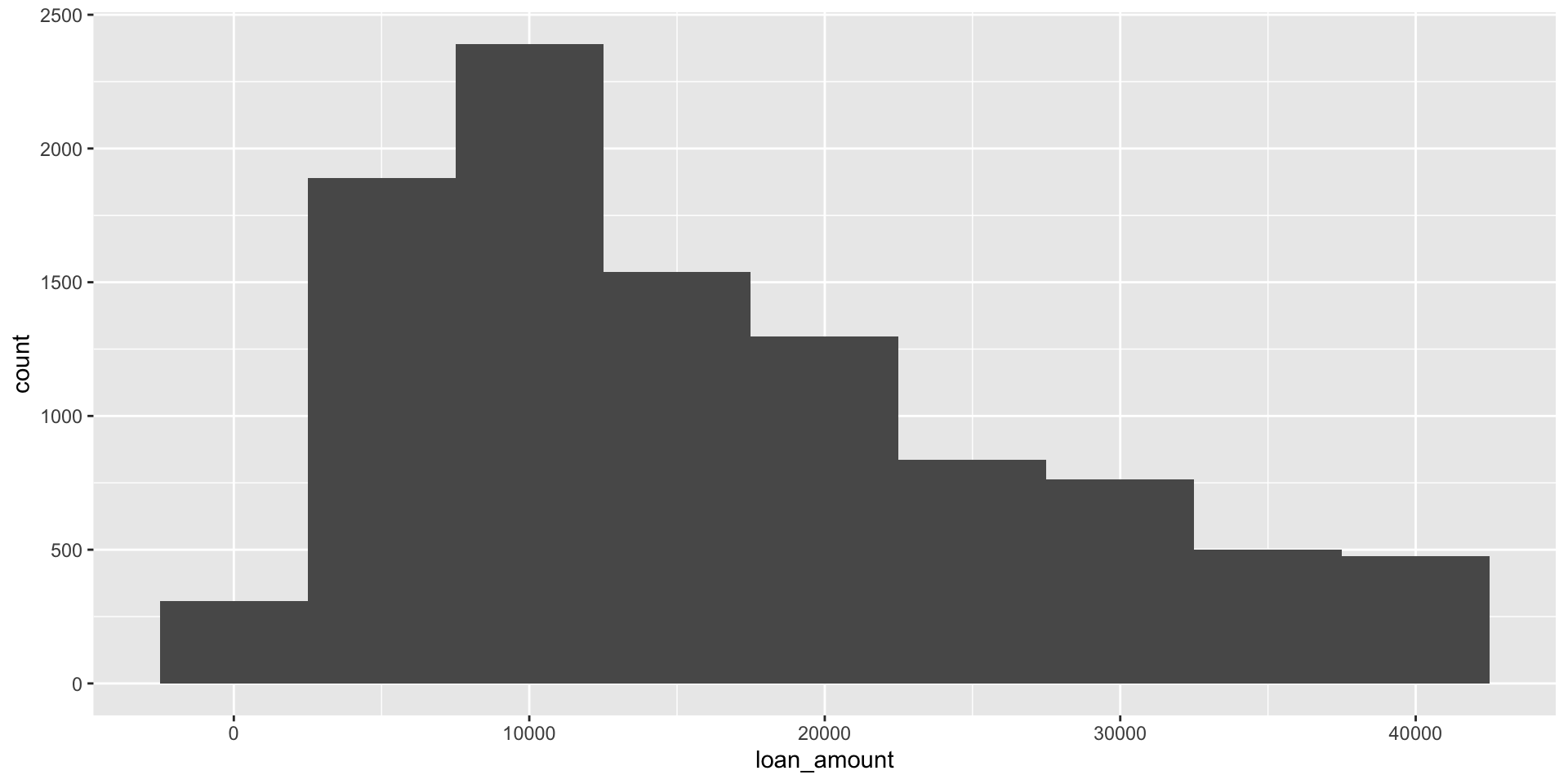
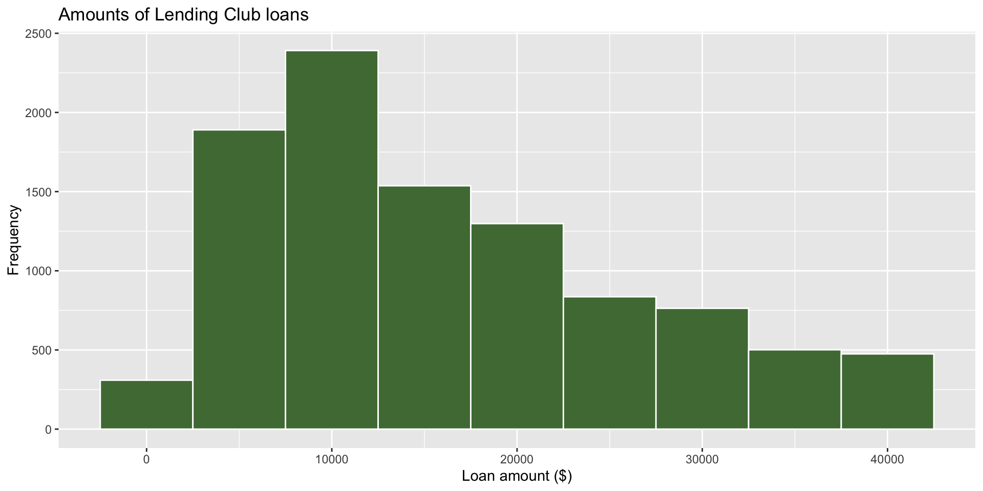
Histogram
`stat_bin()` using `bins = 30`. Pick better value `binwidth`.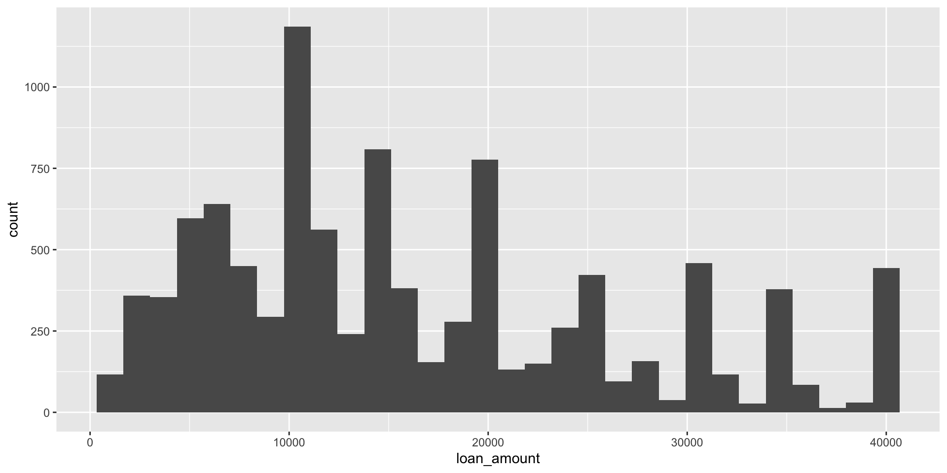
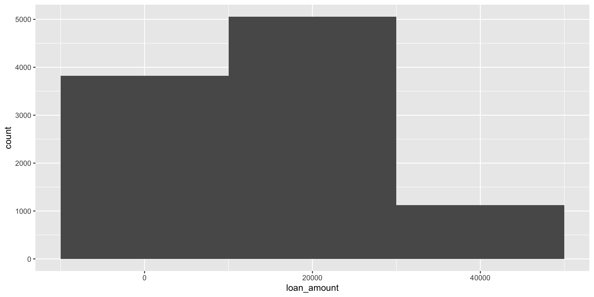
Histograms and binwidth
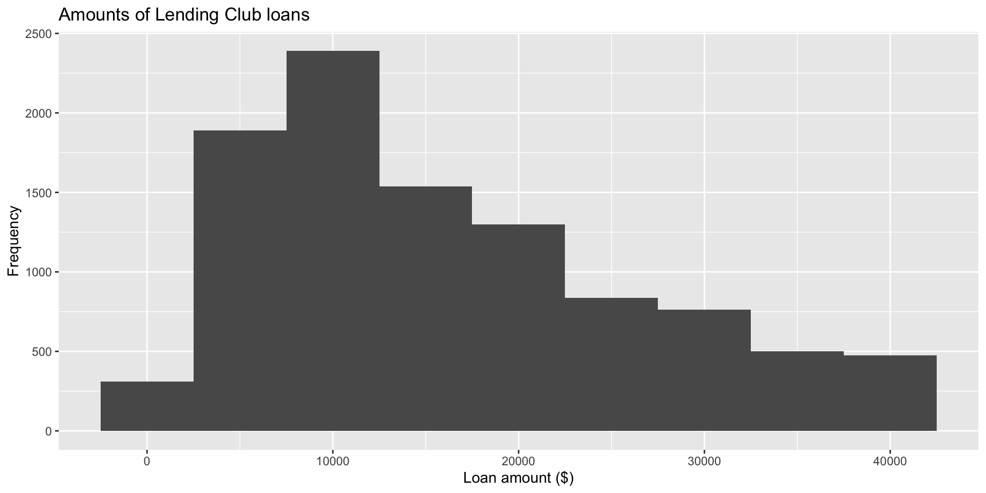
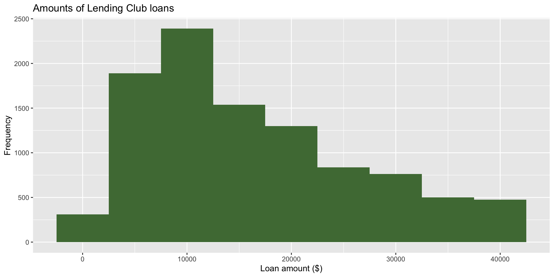
Customizing histograms
Add labels using labs()
Fill in geom_*
Color in geom_*
Fill by a categorical variable
facet_wrap
facet_wrap(~ homeownership, nrow = 3)
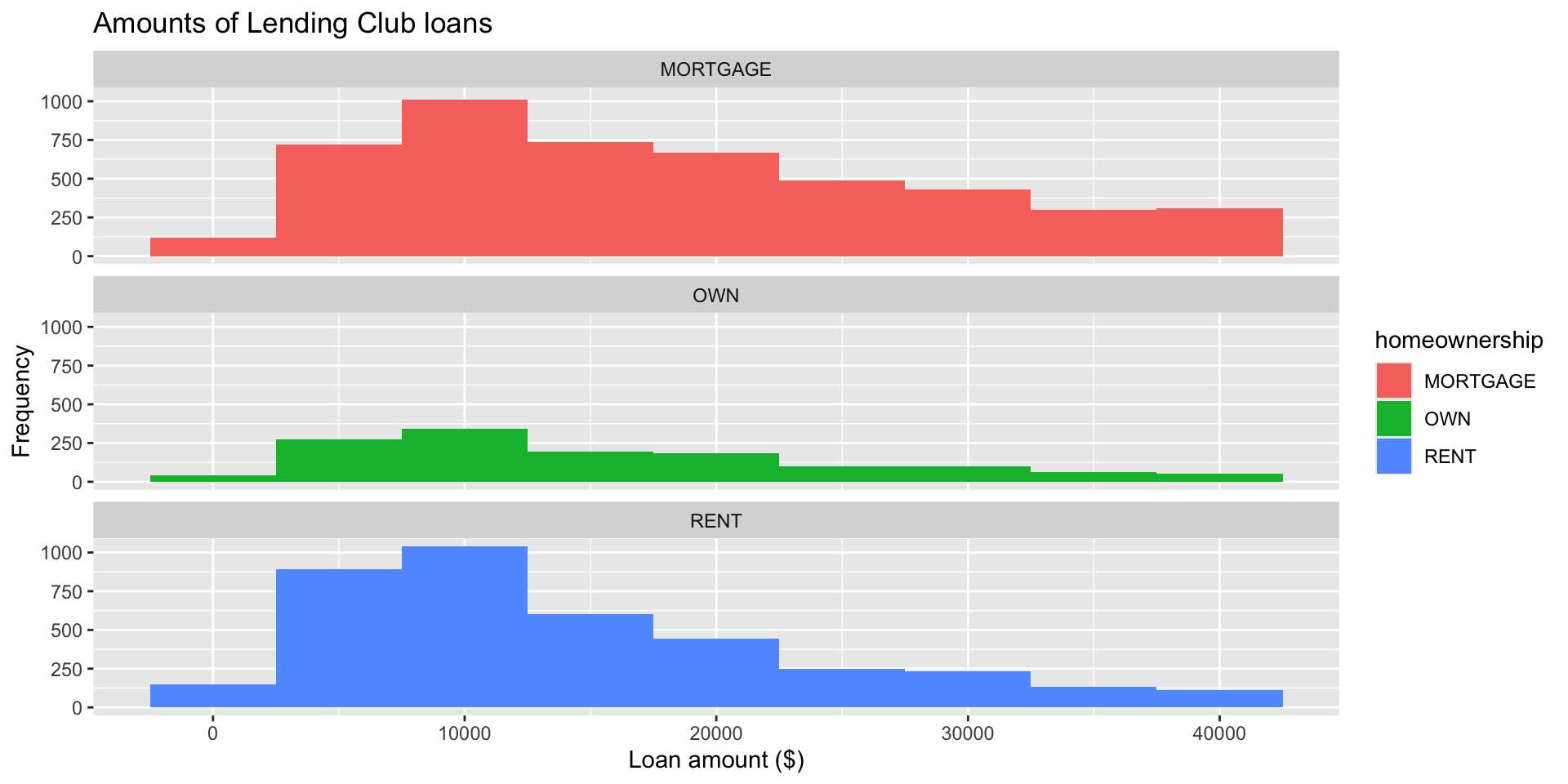
Facet with a categorical variable

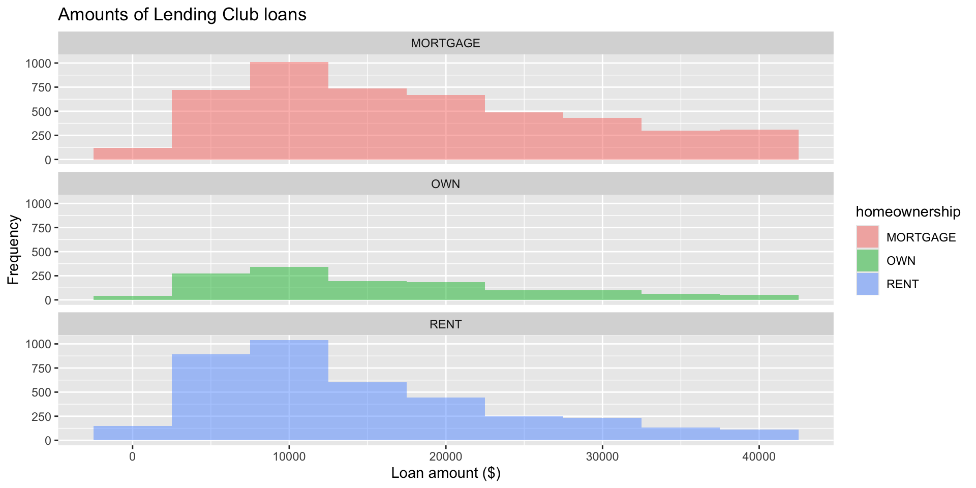
Faceting with transparency in geom_*
geom_histogram(binwidth = 5000, alpha = 0.5)`
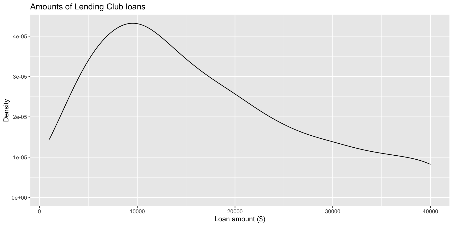
Density plot
Works better for continuous data
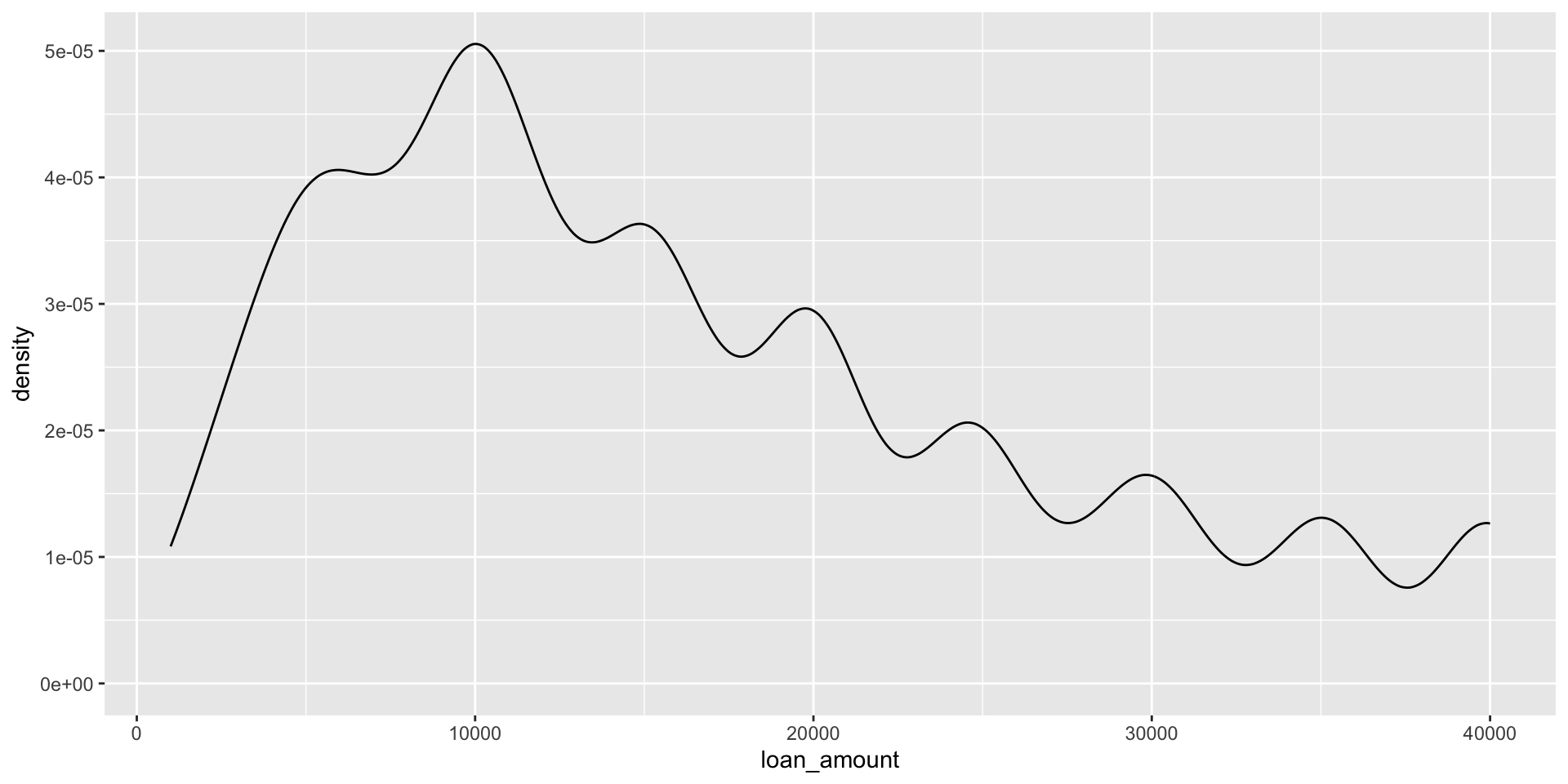
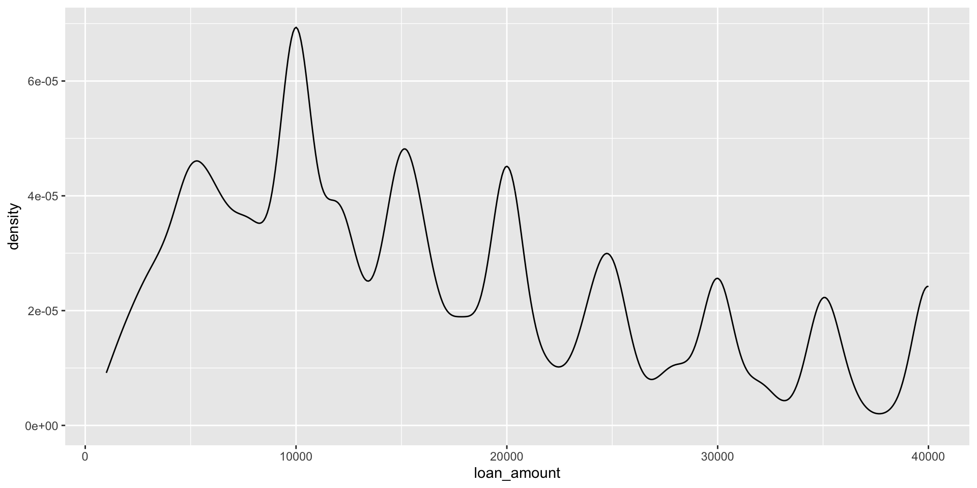
Density plots and adjusting bandwidth

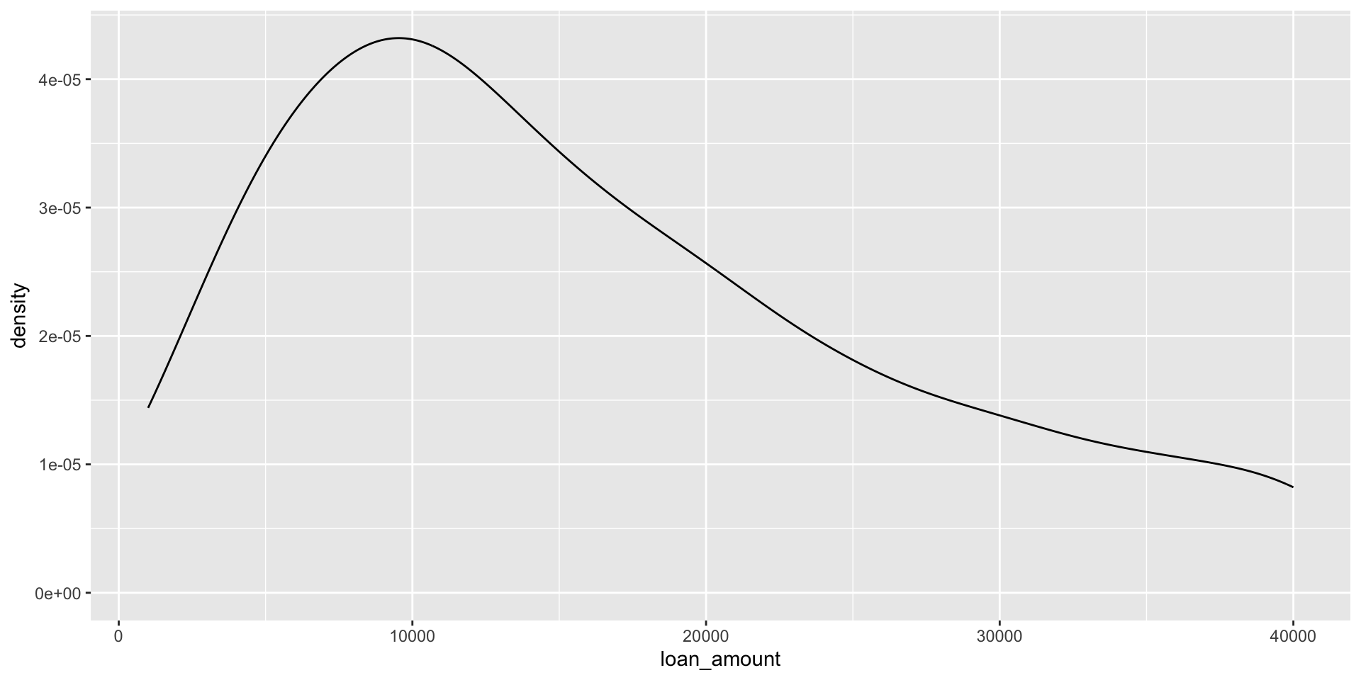
Customizing density plots
Adding a categorical variable
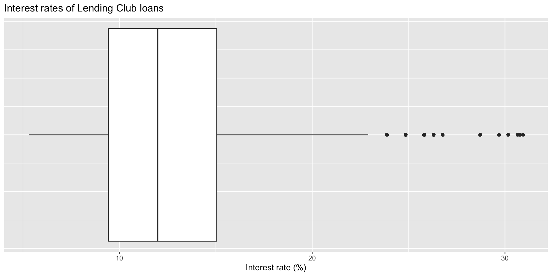
Box plot
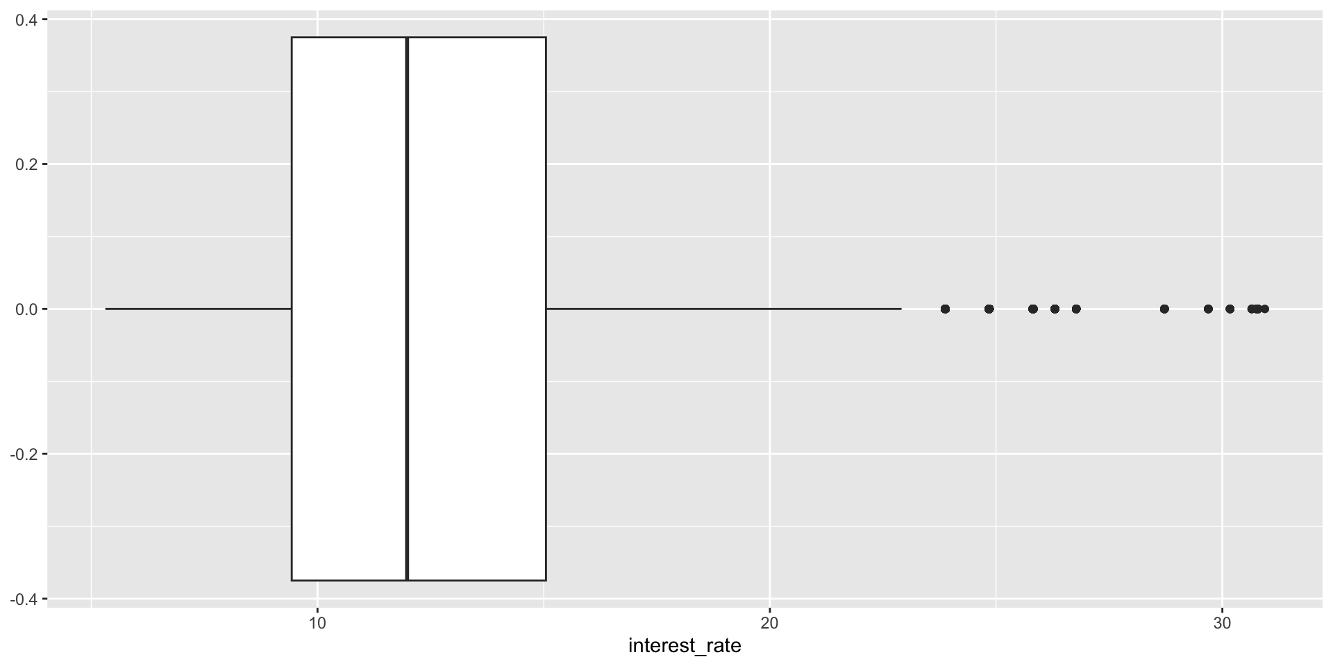
Box plot - flip orientation
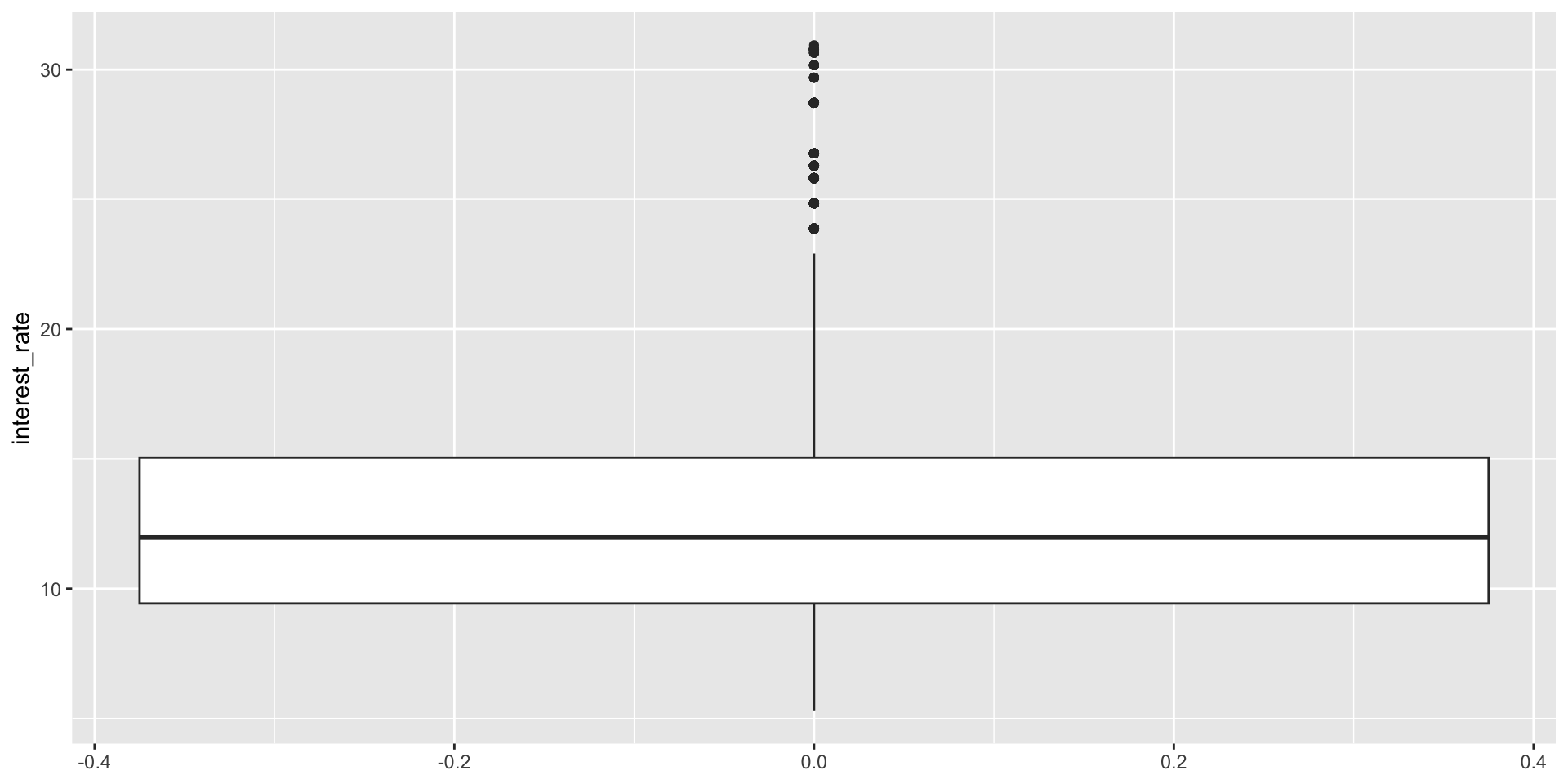
Box plot and outliers
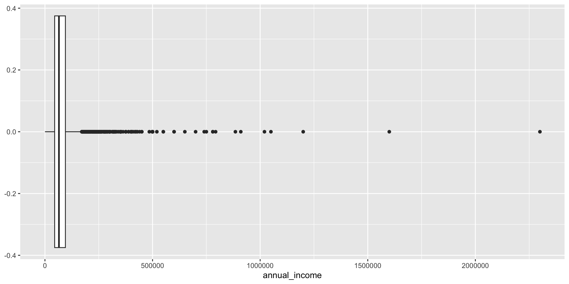
Customizing box plots
Side-by-side box plots
Interest rate by housing tenure (own, own with mortgage, rent)
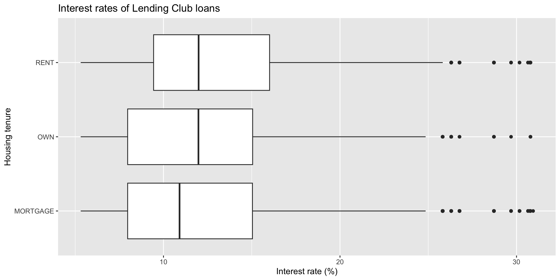
Adding a categorical variable
Scatterplot