Rows: 10,000
Columns: 55
$ emp_title                        <chr> "global config engineer ", "warehouse…
$ emp_length                       <dbl> 3, 10, 3, 1, 10, NA, 10, 10, 10, 3, 1…
$ state                            <fct> NJ, HI, WI, PA, CA, KY, MI, AZ, NV, I…
$ homeownership                    <fct> MORTGAGE, RENT, RENT, RENT, RENT, OWN…
$ annual_income                    <dbl> 90000, 40000, 40000, 30000, 35000, 34…
$ verified_income                  <fct> Verified, Not Verified, Source Verifi…
$ debt_to_income                   <dbl> 18.01, 5.04, 21.15, 10.16, 57.96, 6.4…
$ annual_income_joint              <dbl> NA, NA, NA, NA, 57000, NA, 155000, NA…
$ verification_income_joint        <fct> , , , , Verified, , Not Verified, , ,…
$ debt_to_income_joint             <dbl> NA, NA, NA, NA, 37.66, NA, 13.12, NA,…
$ delinq_2y                        <int> 0, 0, 0, 0, 0, 1, 0, 1, 1, 0, 0, 0, 0…
$ months_since_last_delinq         <int> 38, NA, 28, NA, NA, 3, NA, 19, 18, NA…
$ earliest_credit_line             <dbl> 2001, 1996, 2006, 2007, 2008, 1990, 2…
$ inquiries_last_12m               <int> 6, 1, 4, 0, 7, 6, 1, 1, 3, 0, 4, 4, 8…
$ total_credit_lines               <int> 28, 30, 31, 4, 22, 32, 12, 30, 35, 9,…
$ open_credit_lines                <int> 10, 14, 10, 4, 16, 12, 10, 15, 21, 6,…
$ total_credit_limit               <int> 70795, 28800, 24193, 25400, 69839, 42…
$ total_credit_utilized            <int> 38767, 4321, 16000, 4997, 52722, 3898…
$ num_collections_last_12m         <int> 0, 0, 0, 0, 0, 0, 0, 0, 0, 0, 0, 0, 0…
$ num_historical_failed_to_pay     <int> 0, 1, 0, 1, 0, 0, 0, 0, 0, 0, 1, 0, 0…
$ months_since_90d_late            <int> 38, NA, 28, NA, NA, 60, NA, 71, 18, N…
$ current_accounts_delinq          <int> 0, 0, 0, 0, 0, 0, 0, 0, 0, 0, 0, 0, 0…
$ total_collection_amount_ever     <int> 1250, 0, 432, 0, 0, 0, 0, 0, 0, 0, 0,…
$ current_installment_accounts     <int> 2, 0, 1, 1, 1, 0, 2, 2, 6, 1, 2, 1, 2…
$ accounts_opened_24m              <int> 5, 11, 13, 1, 6, 2, 1, 4, 10, 5, 6, 7…
$ months_since_last_credit_inquiry <int> 5, 8, 7, 15, 4, 5, 9, 7, 4, 17, 3, 4,…
$ num_satisfactory_accounts        <int> 10, 14, 10, 4, 16, 12, 10, 15, 21, 6,…
$ num_accounts_120d_past_due       <int> 0, 0, 0, 0, 0, 0, 0, NA, 0, 0, 0, 0, …
$ num_accounts_30d_past_due        <int> 0, 0, 0, 0, 0, 0, 0, 0, 0, 0, 0, 0, 0…
$ num_active_debit_accounts        <int> 2, 3, 3, 2, 10, 1, 3, 5, 11, 3, 2, 2,…
$ total_debit_limit                <int> 11100, 16500, 4300, 19400, 32700, 272…
$ num_total_cc_accounts            <int> 14, 24, 14, 3, 20, 27, 8, 16, 19, 7, …
$ num_open_cc_accounts             <int> 8, 14, 8, 3, 15, 12, 7, 12, 14, 5, 8,…
$ num_cc_carrying_balance          <int> 6, 4, 6, 2, 13, 5, 6, 10, 14, 3, 5, 3…
$ num_mort_accounts                <int> 1, 0, 0, 0, 0, 3, 2, 7, 2, 0, 2, 3, 3…
$ account_never_delinq_percent     <dbl> 92.9, 100.0, 93.5, 100.0, 100.0, 78.1…
$ tax_liens                        <int> 0, 0, 0, 1, 0, 0, 0, 0, 0, 0, 0, 0, 0…
$ public_record_bankrupt           <int> 0, 1, 0, 0, 0, 0, 0, 0, 0, 0, 1, 0, 0…
$ loan_purpose                     <fct> moving, debt_consolidation, other, de…
$ application_type                 <fct> individual, individual, individual, i…
$ loan_amount                      <int> 28000, 5000, 2000, 21600, 23000, 5000…
$ term                             <dbl> 60, 36, 36, 36, 36, 36, 60, 60, 36, 3…
$ interest_rate                    <dbl> 14.07, 12.61, 17.09, 6.72, 14.07, 6.7…
$ installment                      <dbl> 652.53, 167.54, 71.40, 664.19, 786.87…
$ grade                            <ord> C, C, D, A, C, A, C, B, C, A, C, B, C…
$ sub_grade                        <fct> C3, C1, D1, A3, C3, A3, C2, B5, C2, A…
$ issue_month                      <fct> Mar-2018, Feb-2018, Feb-2018, Jan-201…
$ loan_status                      <fct> Current, Current, Current, Current, C…
$ initial_listing_status           <fct> whole, whole, fractional, whole, whol…
$ disbursement_method              <fct> Cash, Cash, Cash, Cash, Cash, Cash, C…
$ balance                          <dbl> 27015.86, 4651.37, 1824.63, 18853.26,…
$ paid_total                       <dbl> 1999.330, 499.120, 281.800, 3312.890,…
$ paid_principal                   <dbl> 984.14, 348.63, 175.37, 2746.74, 1569…
$ paid_interest                    <dbl> 1015.19, 150.49, 106.43, 566.15, 754.…
$ paid_late_fees <dbl> 0, 0, 0, 0, 0, 0, 0, 0, 0, 0, 0, 0, 0…Visualizing categorical data (and more aesthetics)
Intro to Data Analytics
Data: Lending Club
Thousands of loans made through the Lending Club, a platform that allows individuals to lend to other individuals
Not all loans are created equal – ease of getting a loan depends on (apparent) ability to pay back the loan.
Data includes loans made, these are not loan applications

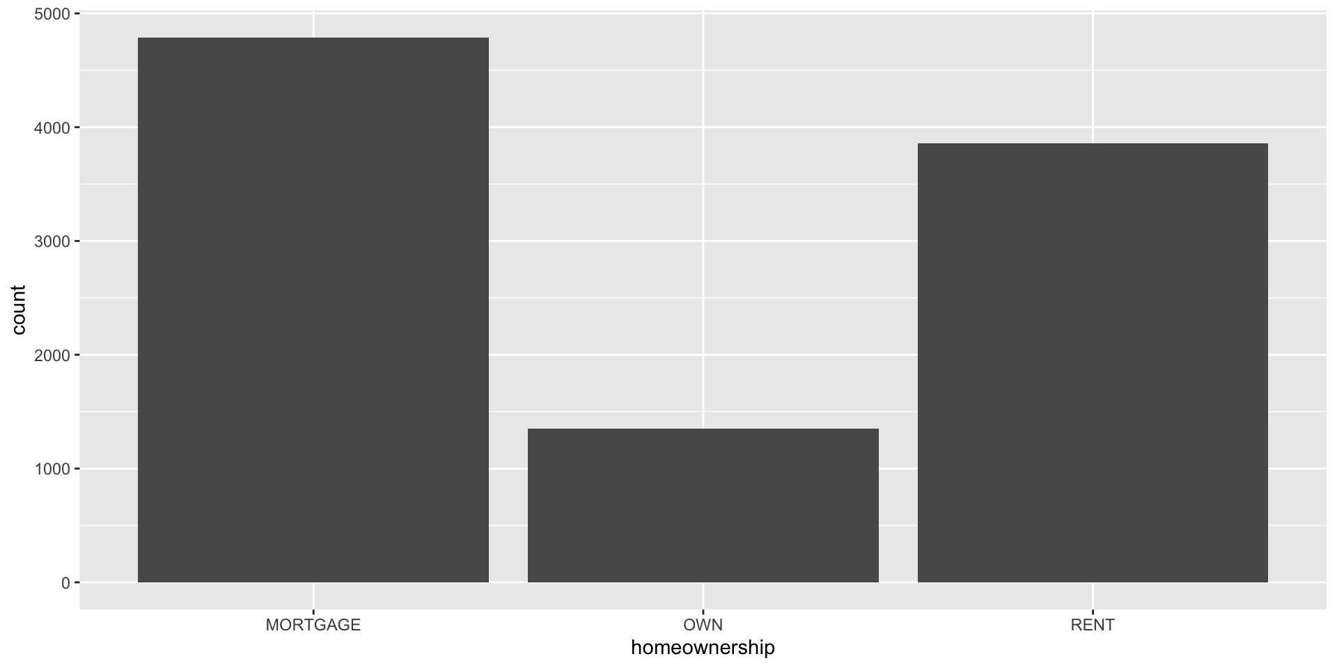
Bar plot
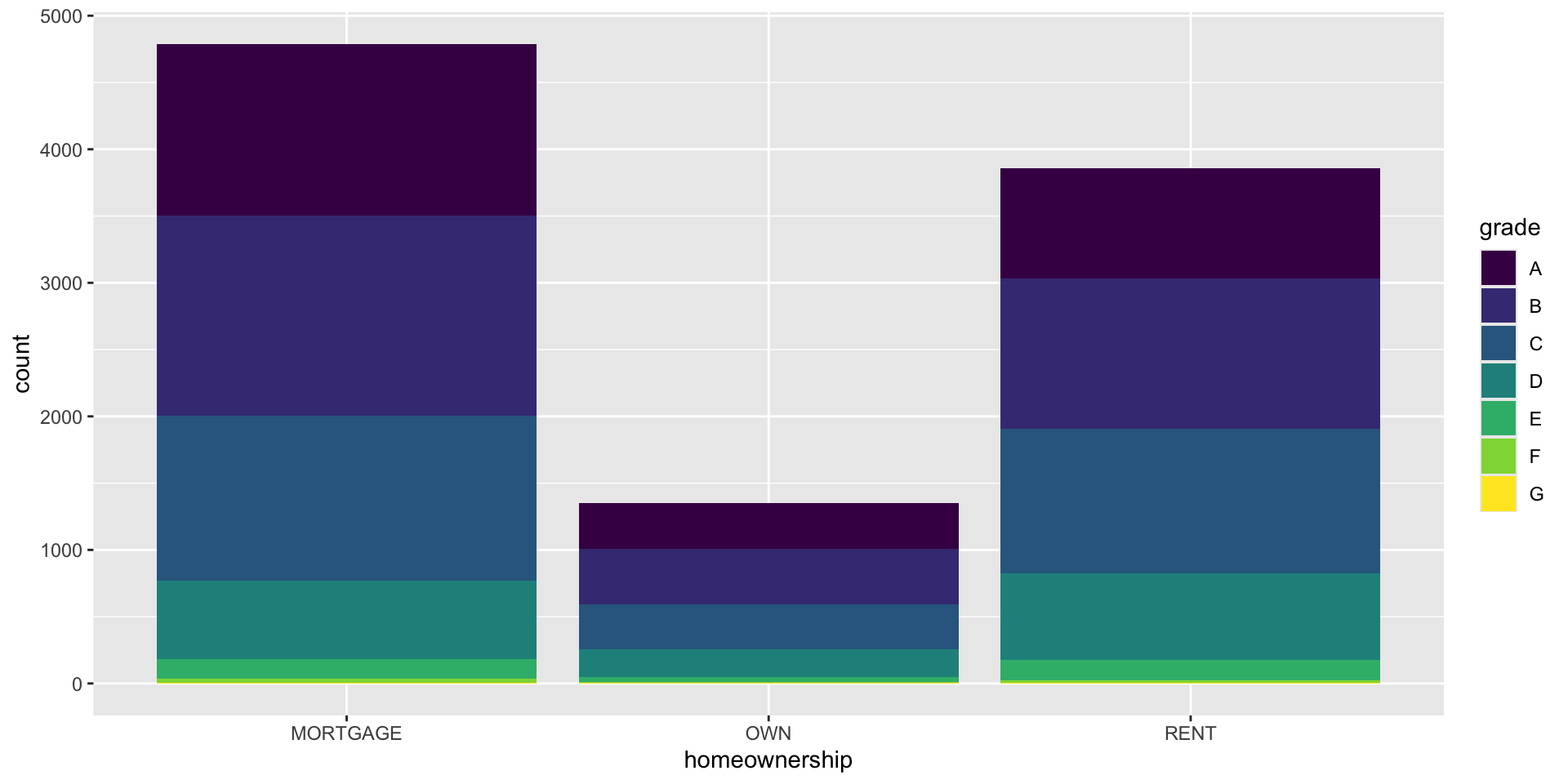
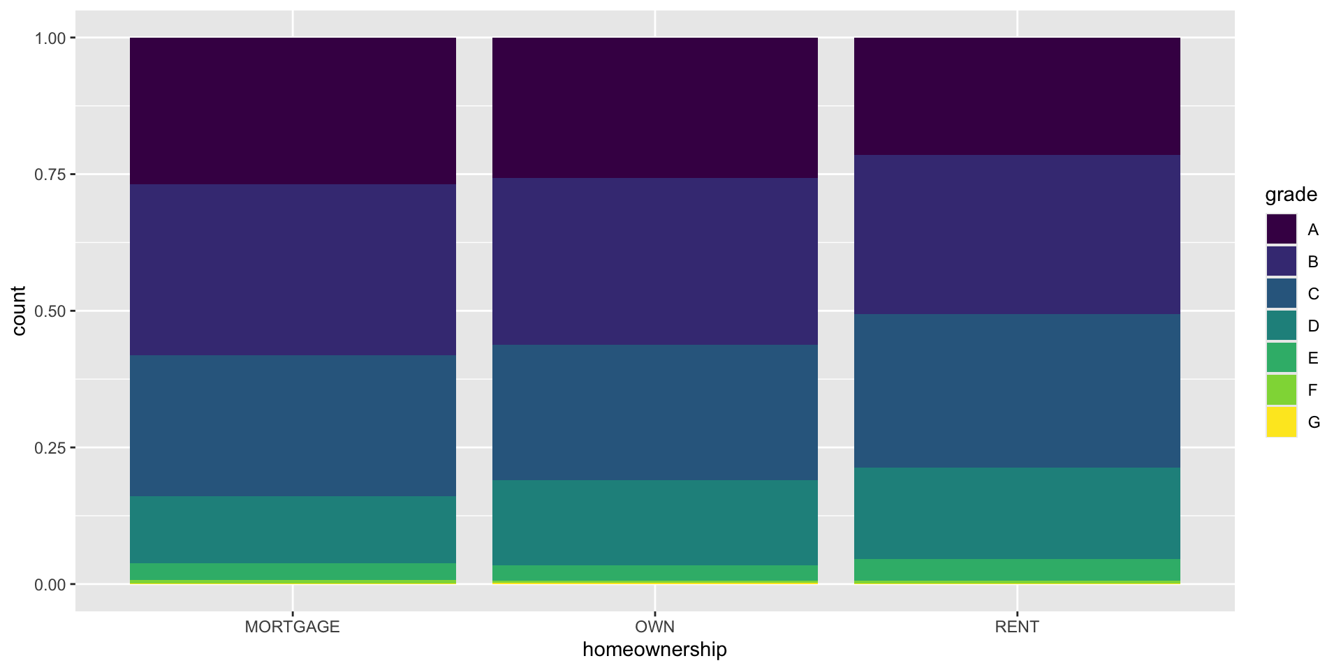
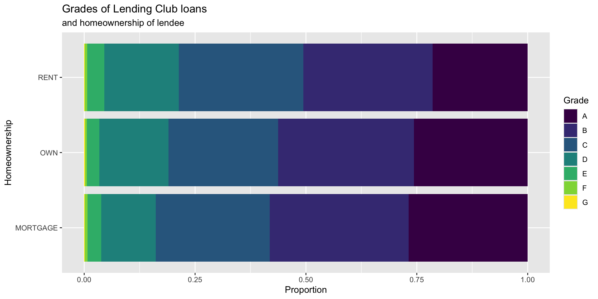
Segmented bar plot

Segmented bar plot
Show proportion.

Bar Plot
Which is a more useful representation for visualizing relationship btwn homeownership and loan grade?
Customizing bar plots
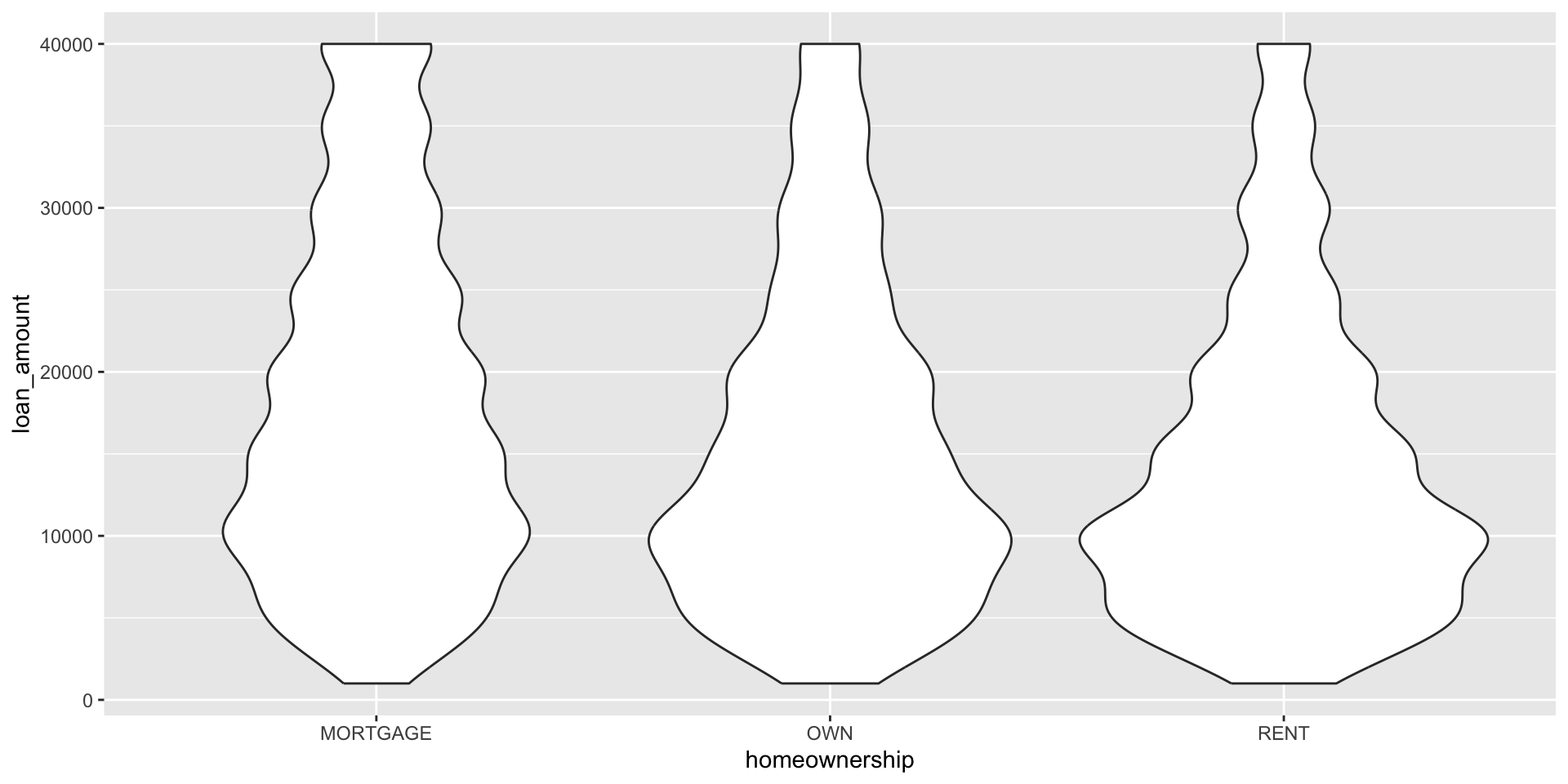
Violin plots
- combine side by side box plots with density plots

Violin plots
- Shows peaks in the data
- For multimodal distributions (those with multiple peaks)
Learn more:
Violin plots
We can add more information to our violin plots to communicate more about the numerical distribution. In the plot below we add a boxplot within the violin.
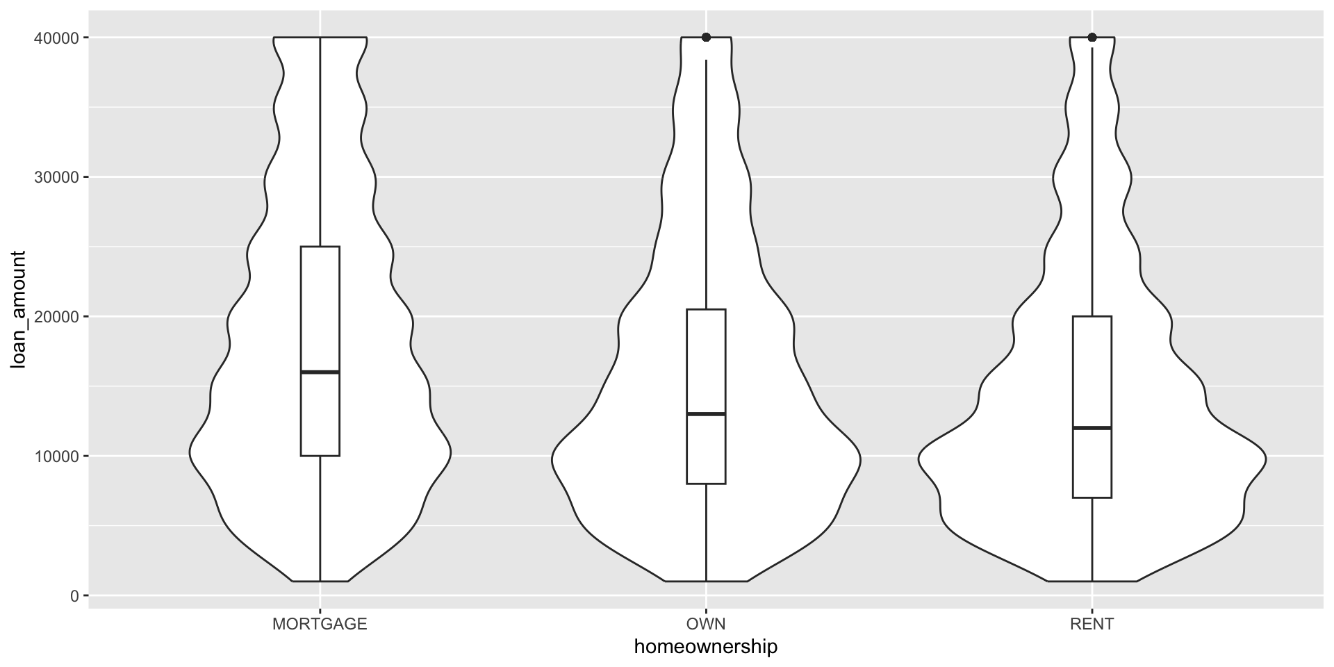
Why did we choose a box plot in this case? What about the distributions shown in the violin geom point us towards displaying the median and IQR?
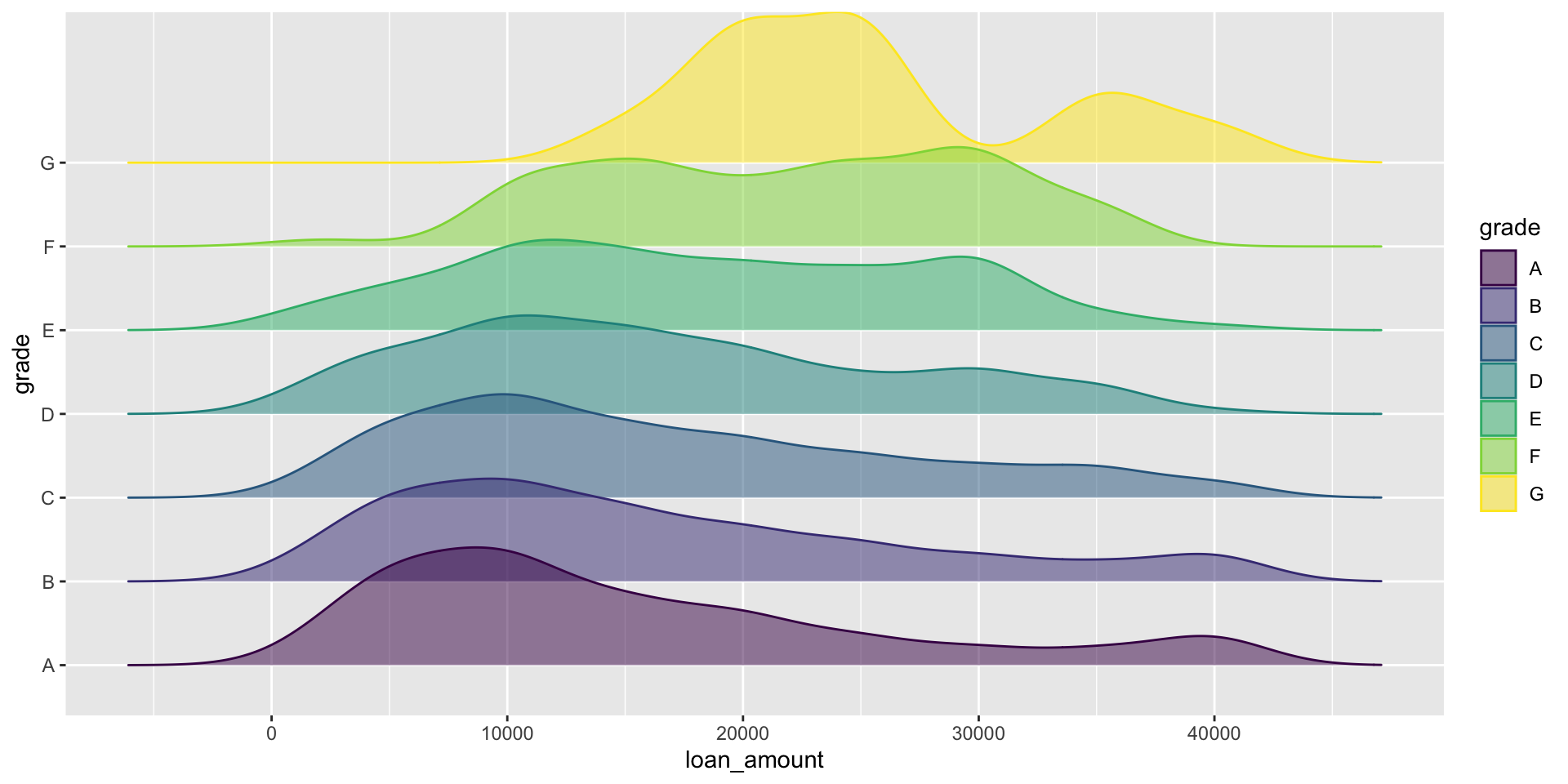
Ridge plots